
Smooth a C-Scan in CIVA ET
In order to increase the resolution a posteriori of a defect response result in CIVA Eddy Current, the user might wish to smooth a simulated C-Scan. It can help to present the results in a more understandable way while limiting the amount of calculation points and time. Of course, as smoothing is based on an interpolation of the available results, the user has to pay attention to have calculated enough points, in order to avoid introducing artifacts in the smoothed C-Scan. But it might also be useful to test through simulation if one signal will be correctly defined after interpolation, in order to determine the number of necessary acquisition steps and the relevant testing speed for a given probe and a given expected type of defect.
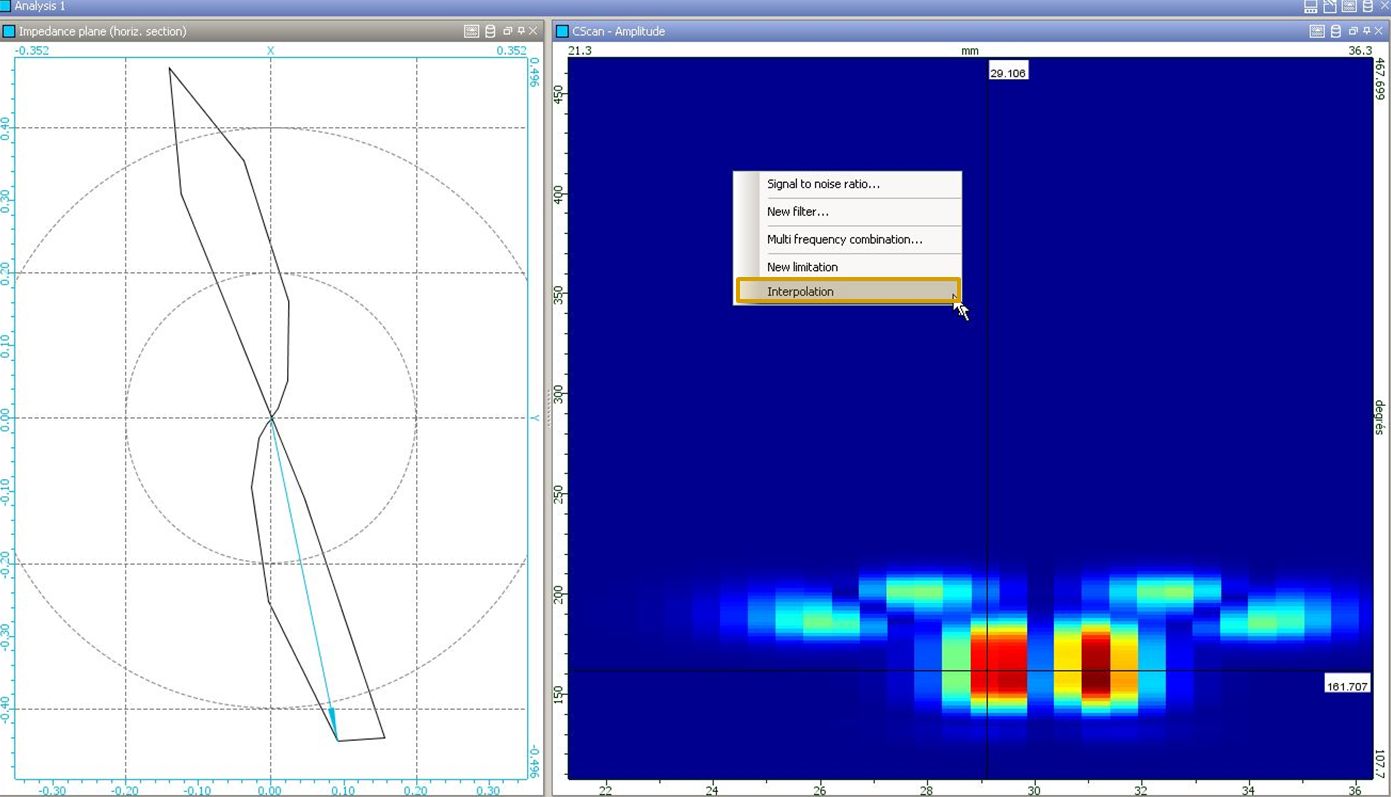
To smooth a C-Scan in CIVA ET, right click on the raw C-Scan then select “Interpolation”. It is different from the smoothing of a field computation image (UT or ET) which is done from the “Image Tools” toolbar on the top of the image.
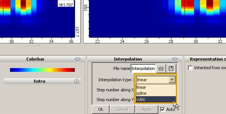
Then, the C-Scan is duplicated in the current page and, in the toolbox at the bottom of the window, 3 interpolation functions are proposed to the user: Linear, Spline and Cubic (actually Cubic Spline). Cubic Spline algorithm is quite popular as an interpolation function; this choice is sometimes detailed in analysis procedures.
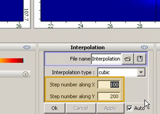
Once the algorithm is selected, the results are interpolated and represent a certain number of points defined by the user along each axis of the C-Scan. The more points you have, the thinner resolution you get. Different results are presented below for a different amount of points.
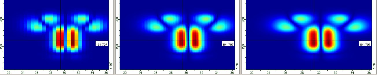
Raw results (30*200 points), interpolation 60*200 points, interpolation 200*400 points
In addition to the Smoothed C-Scan, CIVA ET creates in the meantime a full set of data in a second analysis page. Therefore, the user can also display the associated curves based on the same interpolation: Impedance plane, X and Y channels, Amplitude and Phase curves.
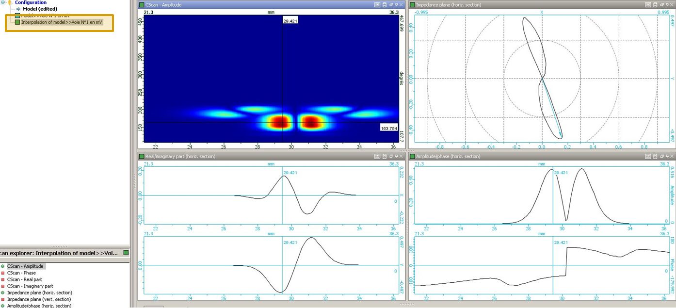
A second analysis page is created in the same project with all smoothed data