Setting and optimizing the time gate and ROI in the CIVA UT FEM module

Computation time is a critical aspect of simulations based on Finite Element Models (FEM), particularly in the “FE Beam Computation” and “FE Inspection Simulation” modules.

The user can reduce computation time by optimizing the following key parameters:

• Time gate
• ROI (Region Of Interest; area in which the FE mesh is generated)
• Mesh quality (see the Mesh quality assessment in CIVA UT FEM module tip)

Integrated tools in CIVA are available to help users efficiently set the time gate and ROI. The following sections describe how to operate them, along with best practices and tips:

 

Time Gate

Objective

A larger time gate results in longer computation times. The “Tmin” parameter has no impact on computation time, as the FE calculation always starts upon entry into the specimen. Reducing computation time via the time gate therefore consists in minimizing “Tmax” as much as possible.

 

Step 1 – Automatic setup (for fast/2D computations)

• Select the mode to consider (L, T, or L+T).
• Select the number of skips on specimen to consider.
• Tip: “0” skip is a suitable setting for direct inspections and/or corner echo inspections located on the backwall of the part (on the left of the figure below). Indeed, CIVA includes a margin in the estimated gate to account for corner echoes. For surface-breaking defects inspected after one backwall skip, a value of “1” skip should be used (on the right of figure below).

 

 

• Click “Estimate gate”: “Tmin” and “Tmax” are automatically computed based on the settings registered previously.

 

Step 2 – Optimization (for long/3D computations)

• Tick time-of-flight visualization in the “Ray path display” tab (located in the toolbox below the 3D view).
• Enable “Round-trip” option, then adjust the displayed time-of-flight value using the slider, or enter manually a value in the tab.

 

 

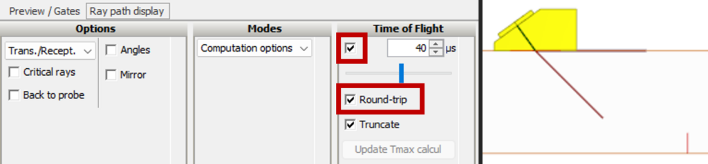
• Tip 1: By adjusting the displayed time-of-flight, it is possible to identify a value where the round-trip ray path reaches the target flaw, while remaining below the automatically estimated time gate limit.
• Tip 2: First, run the current FEM configuration using classical semi-analytical models (which are significantly faster than FE computations). This helps validate the value of the previously optimized time gate. For example, verify that flaws echoes are correctly visible and not truncated by the gate, across all probe positions or PA delay laws depending on the scan type. This semi-analytical computation can be performed in 2D mode (as the analysis is not quantitative) and can be compared to a reference computation using CIVA’s automatic gate.
• NB: Switching between both modules is straightforward; when editing a FEM model, open the CIVA Desk and load the current configuration in the “Inspection Simulation” module from the CIVA UT tile. Simulation settings, including the time gate, are preserved during this switch.

 

ROI (Region Of Interest)

Objective

As with the time gate, a larger ROI results in longer computation times. It is essential to restrict it (and meshing) to the region of interest.

 

Step 1 – Automatic setup (for fast/2D computations)

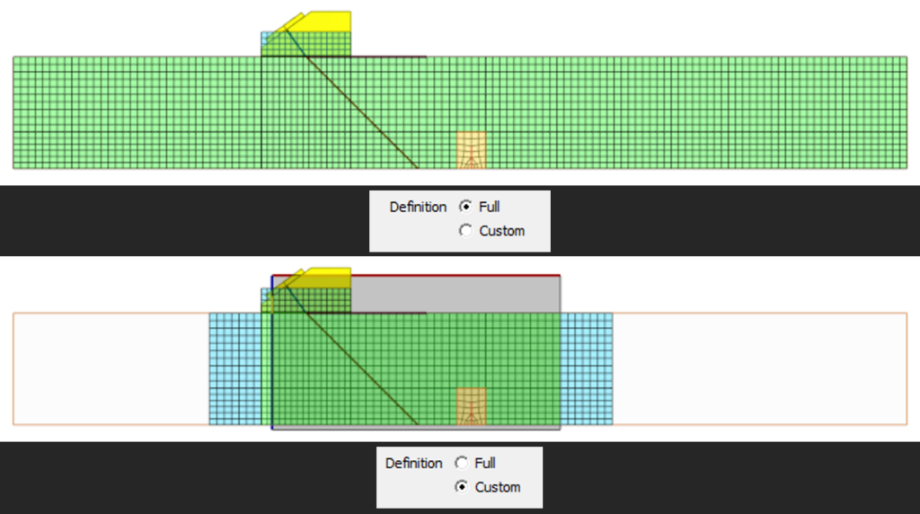
• If not selected by default, set ROI definition to “Custom”. If ROI is set to “Full”, CIVA meshes the entire specimen, which is rarely necessary and leads to significant computation time (especially for large components).

 

 

• NB: The automatic ROI estimation tool depends on the previously defined time gate. Therefore, the gate must at least be set using the automatic estimator and be consistent with the current configuration.
• Select the “Mechanical link” ROI, relative to either the “Specimen” or the “Probe”. This choice can impact computation time and will depend on the inspection setup (see Step 2 – optimization for the ROI).

 

 

• Click “Estimate ROI”. ROI size and position are updated automatically; this change is also visible in the 3D view.

• NB: The out of inspection plane ROI extension is estimated based on the probe width. In 3D cases for which the flaw is larger than the probe, it may be necessary to manually adjust ROI width to fully cover the flaw width (or at least the UT beam width in that plane).

 

Step 2 – Optimization (for long/3D computations)

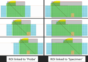
• ROI linked to the “Probe”: recommended when mechanical scanning is enabled. ROI size is estimated based only on the ray path (or UT beam), without necessarily covering the target flaw.
• ROI linked to the “Specimen”: ROI size is tied to both flaw and probe position (based on the furthest probe position relative to the flaw in case of a mechanical scanning). This may result in larger ROIs than with the “Probe” linkage, without this being necessary to accurately model beam/flaw interactions. However, in some configurations, it can be beneficial for the ROI not to follow probe scanning.
• Tip: It is recommended to test both options to select the most appropriate one depending on the testing configuration. By visualizing the mesh for multiple probe positions during scanning, it is possible to ensure that the mesh correctly covers all relevant elements (ray path and target flaw).
• Move the probe in the 3D view to the position of interest, then click “Mesh level 1” using the “Current position”. Repeat this action for different probe positions and compare meshes depending on ROI linkage type (illustration below).