Inclusion in water - phased-array - Configuration with delay law

As for the configurations without delay laws, a reference has been chosen for each active aperture for the relative amplitudes calculation. It has been obtained comparing experimental and simulation results of a  Ø2 mm SDH echo at low depth on the calibration block obtained varying the water path. No delay law has been parameted for the reference. As the far field is located at an important distance from the probe surface, the echodynamic curves comparison has been done on 380 mm (maximal distance allowed by the testing bench).

Depending on the active aperture, the configuration and the following calibration SDH has been chosen :

• Aperture of 20 elements : SDH at 12 mm depth, 151 mm water path (same reference than the configuration without delay law)
• Aperture of 32 elements : SDH at 24 mm depth,  201 mm water path
• Aperture of 48 elements : SDH at 68 mm depth, 261 mm water path
• Aperture of 64 elements : SDH at 68 mm depth, 261 mm water path

The reason why the reference SDH depth increases as a function of the aperture is due to the fact that the SDH at lower depth are not exploitable because of a surface echo very extended in time mixing with the SDH echo.

Amplitude/distance curves comparison is presented Figure 30. It shows a good prediction of the SDH amplitude for all apertures to within 2 dB.

Note : experimental amplitudes appear noisy on the figure. It is either because of parasite signals coming from the acquisition chain, either « phantom » echoes related to the great numerisation depth that is added to the real echo. Some of those indications have been suppressed on the figure, that's why empty zones appear.

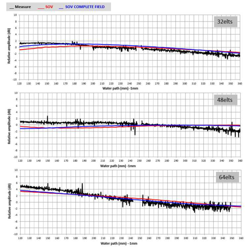
Figure 30 : Comparison of  measured and with SOV, SOV-COMPLET simulated amplitude/distance curves, Ø2 mm SDH at 24 mm and 68 mm depth in the ferritic steel calibration block. Phased array probe, 5 MHz,  Comparaison des courbes amplitude/distance mesurées et simulées avec SOV, SOV-COMPLET, TGØ2mm à 24mm et 68mm de profondeur dans le bloc d’étalonnage en acier ferritique. Capteur multiéléments 5MHz, 32, 48 and 64 elements apertures, focalisation at 33 mm in water.  

The Figure 31 presents the simulated field emitted by the phased array probe in water with a set of delay laws allowing a focalisation at 33 mm in water at L0°. The delay laws has been calculated for the 4 active apertures: 20, 32, 48 and 64 elements. Under each beam cartography (with same dimensions for all apertures: 10 x 60 mm) are represented the amplitude/distance curve extracted at the aperture center and, to the right hand side, the profile in the perpendiculary plan to the distance corresponding at the maximal amplitude.

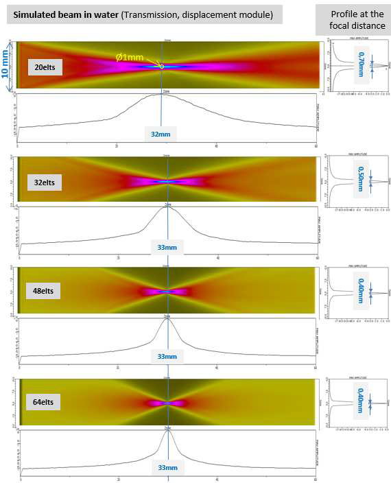
Figure 31 : Simulation with CIVA of the field emitted by the probe in water with a focal law of 33 mm in water for 4 different active apertures:  20, 32, 48 and 64 elements. Phased array probe, 5 MHz.

The maximal amplitudes positions as a function of the active aperture and the focal spot width at -3 dB are written in the table 5.

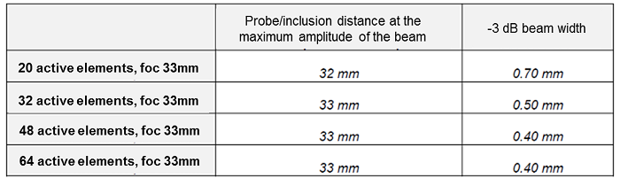
Tableau 5 : Probe/inclusion distances corresponding to the beam maximal amplitude emitted on the probe axis and focal spot width as a function of the active aperture. Phased array probe with 20, 32, 48 and 64 active elements. focal law at 33 mm depth in water.  

The Figure 32 shows the beam profile example following the probe center obtained for an aperture of 32 elements and a focal law allowing a focalisation at 33 mm in water at L0°. Field cartographies at fixed water path in the perpendiculary plane have also been computed and are presented at the bottom of the figure.

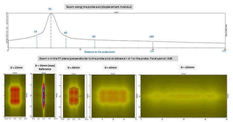
Figure 32: CIVA simulation of the field emitted by the phased array probe in water.  On the top: beam profile along the probe axis showing a maximum at a distance of 33 mm from the probe. On the bottom, cartographies (10 mm x 20 mm, 20 mm x 20 mm and 40 mm x 20 mm) of the beam the planes perpendicular to its axis at different probe distances. Comparable amplitudes (ref = beam maximal amplitude obtained at D = 33 mm). Phased array probe with 32 active elements, focalisation at 33 mm in water, 5 MHz. 

 

amplitude/distance curves

Experimental and with the three models SOV, SOV_COMPLETE and SPECULAR simulated amplitude/distance curve comparisons are presented fir the 4 active apertures (20 and 32 elements on the Figure 33; 48 and 64 elements on the figure 34) and a focal law allowing a focalisation at 33 mm in water. The gaps between dmaxEXPERIMENTAL and dmaxCIVA are indicated on the table 6.

Aperture of 20 elements:

A good agreement is obtained between the experiment and the simulation. The specular echo maximal position as well as its amplitude relatively to the reference SDH echo are well predicted with the three models. A better prediction is obtained with the « ray » model after the focal zone (maximal gaps reache 2 dB).

Aperture of 32 and 48 elements:

We also observe a good prediction fo the three models on the amplitude evolution and the maximal amplitude position of the specular echo. The maximal differences are about 2/3 dB. As for the 20 elements aperture, we observe a better prediction with the SOV-COMPLETE and SPECULAR models after the focal zone. However it exists, after the focal zone, un slight amplitude oscillation that does not appear in the experiment. The amplitudes differences do not exceed 2 dB.

Aperture of 64 elements:

This case shows the contribution of SOV-COMPLETE and SPECULAR models on the amplitude prediction of the inclusion echo as a function of the water path. Indeed, outside the focal law, the simulated amplitudes with the SOV model tend to be underestimated. The maximal differences observed between experiment and model predictions reach 5/6 dB. Between experiment and SOV-COMPLETE and SPECULAR models, those differences are lower than 2 dB.

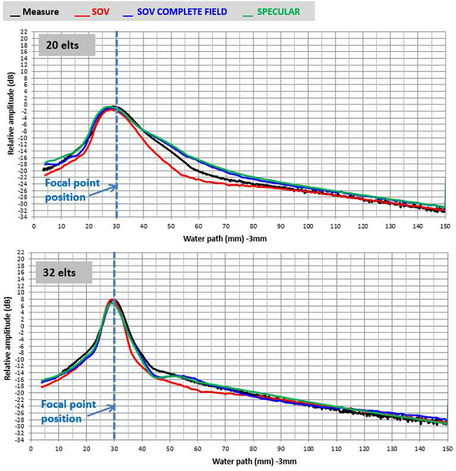
Figure 33: Comparison of measured and with SOV, SOV_COMPLETE and SPECULAR models simulated amplitude/distance curves in water on an Ø1 mm inclusion, apertures of 20 and 32 elements, focalisation at 33 mm in water. The vertical lines correspond to the focal point position. Phased array probe, 5 MHz.  

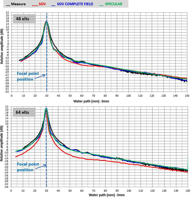
Figure 34: Comparison of measured and with SOV, SOV_COMPLETE and SPECULAR models simulated amplitude/distance curves in water on an Ø1 mm inclusion, apertures of 48 and 64 elements, focalisation at 33 mm in water. The vertical lines correspond to the focal point position. Phased array probe, 5 MHz.  

 

The « dmax » distance, at which the echo amplitude is maximal is well predicted with all models and for all apertures. The gaps do not exceed 1 mm.

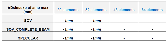
Tableau 6: Differences measure/CIVA between the probe/inclusion distances of the previous table. Numbers written in bold correspond to not restrained cases in CIVA. Focalisation at 33 mm depth in water. Phased array probe, 5 MHz.   

 

The A-scans of the experimental and with SOV and SOV_COMPLETE models simulated inclusion echoes are represented on the Figure 35 for two distances between the probe and the inclusion. For more clarity, only the first ball echo (specular echo) is presented. On the other hand, as the A-scans obtained with the SPECULAR and SOV_COMPLETE models are similar, only the SOV_COMPLETE A-scan is represented.

The superimposition of A-scans show a good prediction of the echoes signal shape for the different cases. At a water path of 103 mm, the SOV_COMPLETE model seems to be more accurate concerning the frequency and the signal shape relatively to the SOV model with a plane wave approximation.

 

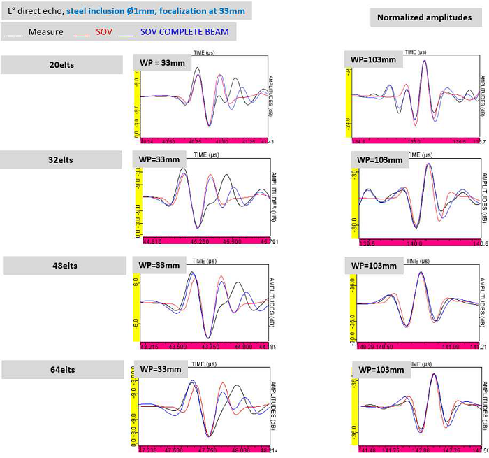
Figure 35: Comparison of measured and with SOV and SOV_COMPLETE simulated A-scans on a Ø1 mm inclusion. Focalisation at 33 mm depth in water. Phased array probe, 5 MHz.  

 

Cartographies in the XY plane

The experimental and with the 3 models simulated XY echodynamic curves have been extracted at the focal point position in water (33 mm) for all active apertures. The Figure 36 corresponds to the apertures of 20 and 22 active elements and the Figure 37 corresponds to the aperture of 48 and 64 active elements, along the X axis.

The curves are normalized in amplitude ( max amplitude = 0 dB ) in order to compare the focal widths.

Figure 36: Comparison of experimental and with SOV, SOV_COMPLETE and SPECULAR models along X simulated echodynamic curves on an Ø1 mm inclusion, apertures of 20 and 32 elements, focalisation at 33 mm in water. Phased array probe, 5 MHz. 

 

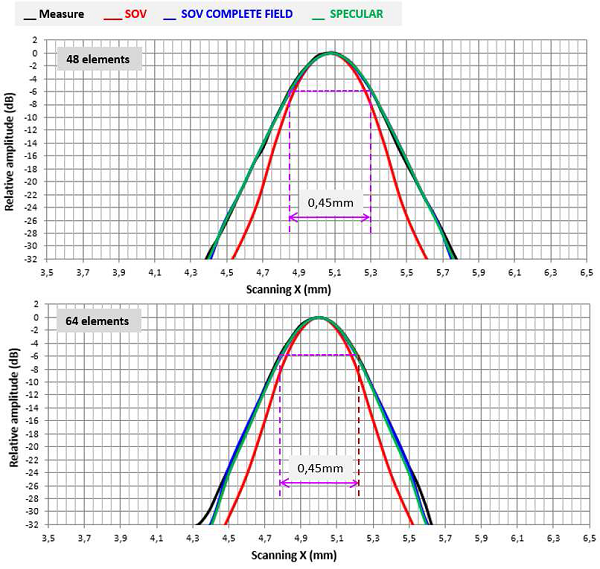
Figure 37:

Comparison of experimental and with SOV, SOV_COMPLETE and SPECULAR models along X simulated echodynamic curves on an Ø1 mm inclusion, apertures of 48 and 64 elements, focalisation at 33 mm in water. Phased array probe, 5 MHz. 

The comparison of experimental results with SOV_COMPLETE and SPECULAR models show a significant improvement of predictions for the most far areas from the probe center. Indeed, the differences reach 2 dB for the maximum even for an observation point located at -32 dB under the maximal amplitude.

The Figure 38 show an exemple of superimposition of the experimental and following Y axis simulated echodynamic curves, extracted at a 33 mm water path and an aperture of 32 active elements. The comparison shows that the 3 models quite well predict the amplitudes. The differences between experiment and simulation do not exceed 2 dB for every models.

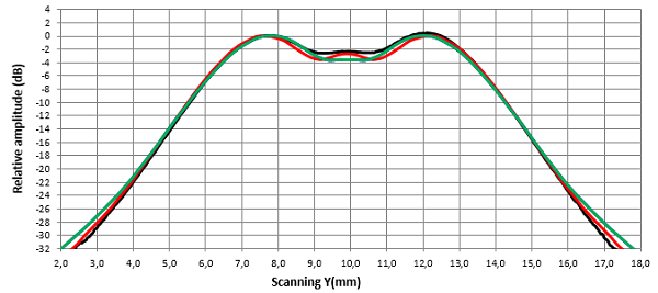
Figure 38: Comparison of experimental and with SOV, SOV_COMPLETE and SPECULAR models along Y simulated echodynamic curves on an Ø1 mm inclusion, apertures of 32 elements, focalisation at 33 mm in water. Phased array probe, 5 MHz. 

 

The differencies between simulated and experimental at -6 dB focal spot width as a function of the active aperture are indicated on Table 7.

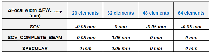
Tableau 7: Differences ( in mm ) between simulations and measures for focal spots at -6 dB along X at distances for which the amplitude/distance curve amplitude is maximal. Simulation results with the 3 models. Focalisation at 33 mm depth in water. Phased array probe, 5 MHz.