
Inclusion in water – single element – 2.25 MHz probe
Summary
- INPUT PARAMETERS IN CIVA
- PROBE ParamEtERs
- INCLUSION ParamEtErs
- WATER ParamEtERs
- REfErence FOR THE AMPLITUDES FOR EXPERIMENTS VS SIMULATED AMPLITUDES
- BEAM OF THE 2.25 mhZ PROBE IN WATER
- REsults obtAINED WITH STEEL INCLUSIONS
- EXPERIMENTAL RESULTS
- EXPERIMENTS/CIVA COMPARISON
- Results obtained with the infinite plan
- ECHOES SPECTRUM OF INCLUSION AND INFINITE PLAN
- EFFECT OF small CHANGEs IN the central frequency
- Synthesis
INPUT PARAMETERS IN CIVA
PROBE ParamEtERs
The diameter of the probe defined in CIVA is the one given by the manufacturer:
- Probe diameter : 6.35mm
The central frequency of the input signal is the nominal frequency given by the manufacturer:
- Central frequency = 2.25 MHz
The two other parameters of the input signal, the bandwidth and phase, are determined by fitting the temporal shapes of the measured and simulated echoes from a reference reflector which CIVA predictions have been validated.
The reference reflector chosen for this probe is a SDH of diameter D = 2mm located at 44mm depth in a steel calibration block. This reference echo has been measured for a water depth of 20mm.
The bandwidth and the phase of the signal are (Figure 14):
- Bandwidth =55%
- Phase = 40°
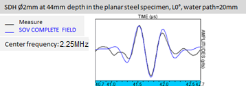
Figure 14 : Superposition after ajustment dof the bandwidth and phase of the signal of experimental A-scans ans simulated ones with COMPLETE_SOV of a Ø2mm SDH located at 44mm depth, waterpath 20mm. Normalized amplitudes. Flat probe Ø6.35mm, 2.25MHz.
INCLUSION ParamEtErs
The inclusions diameters defined in CIVA are the ones provided by the manufacturer:
- Inclusion diameter = 1, 2, 4 and 6 mm
Longitudinal and shear waves velocities in the inclusions couldn’t be measured precisely. However, they were determined thanks to a small parametric study with CIVA by using the fact:
- that a shear wave variation close to 3000m/s (velocity in steel) has an effect on the position and amplitude of the echoes arriving after the specular echo (Figure 15, top).
- that a L wave velocity variation has little effect on the amplitude of these echoes and not only on their positions (Figure 15, bottom)
- that the specular echo does not depend on the values of these velocities (Figure 15)
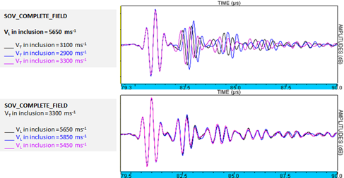
Figure 15 : Simulation results illustrating the effect of a shear wave velocity variation (top) and a L wave velocity variation (bottom) in the Ø2mm inclusion placed in immersion at 60mm waterpath. The effect of the variation of shear wave on the echoes arriving after the specular echo was used to determine the velocity of these waves. Ø6.35mm flat probe, 2.25MHz.
Thus, the speed of T-waves in the inclusion is determined by adjusting the temporal positions of the echoes arriving after the first experimental and COMPLETE_SOV simulated specular echo (Figure 16, top).
The value that has been obtained is:
- vT-steel = 3300 m/s (Figure 16 bottom).
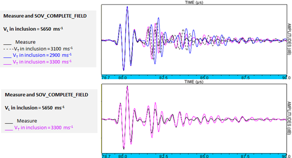
Figure 16 : Superposition of experimental and COMPLETE_SOV model A-scans from the Ø2mm inclusion placed at 60mm from the probe. Top: experimental A-scan and 3 simulated A-scans obtained with 3 different T velocities in the inclusion. Bottom: experimental and simulated A-scans with shear wave velocity for which we obtain the best agreement. Ø6.35mm flat probe, 2.25MHz.
Note : the SOV and COMPLETE_SOV models simulate the same echoes after adjustment (Figure 17). The determined velocity does not depend on the chosen model for simulation.
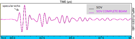
Figure 17 : Superposition of A-scans simulated with SOV and COMPLETE_SOV models of the echo of the Ø2mm inclusion placed at 60mm from the probe. We can see that the specular echo and the following ones do not depend of the model. Flat probe, Ø6.35mm, 2.25MHz.
Then, the L wave velocity in the inclusion was determined by adjstment of the amplitude of the simulated and experimental amplitude echo following the first specular echo (Figure 18 top).
The value that was obtained is (Figure 18 bottom):
- vL-steel = 5850 m/s.
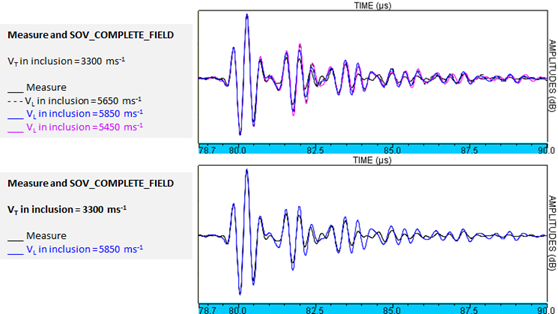
Figure 18 : Superposition of experimental and COMPLETE_SOV model A-scans from the Ø2mm inclusion placed at 60mm from the probe. Top: experimental A-scan and 3 simulated A-scans obtained with 3 different L velocities in the inclusion. Bottom: experimental and simulated A-scans with shear wave velocity for which we obtain the best agreement. Ø6.35mm flat probe, 2.25MHz.
The L and T wave velocities that were determined for the Ø2mm inclusion were used as input data in CIVA for the other inclusion beacuse we suppose that they are identical.
Note: this method for determining the L and T waves velocities in the inclusion is not very accurate and makes the assumption that COMPLETE_SOV model predicts accurately the echoes following the specular one whereas this model is still being validated. Nevertheless we kept this adjustment because it has no consequence for the rest of the study since it concerns the inclusions specular echo which do not depend on the values of these speeds.
WATER ParamEtERs
This velocity was measured sing the successive bounces of a surface echo on an infinite plan.
- vLwater = 1483 m/s
The attenuation in the water has been neglected in simulations with a frequency of 2.25MHz, because it is very small. Moreover, we verified by comparing simulations with and without attenuation that it is has no effect on the probe/reflector distances chosen in this study.
- Attenuation in water neglected for the 2.25 MHz probe
REfErence FOR THE AMPLITUDES FOR EXPERIMENTS VS SIMULATED AMPLITUDES
The reference amplitude for comparison experiment/simulation results is the amplitude of the L0 ° specular echo of the Ø2mm SDH located at 44mm steel depth in the steel calibration block inspected with a waterpath of 20 mm (Figure 14). The amplitudes of the echo obtained with the SOV and COMPLETE_SOV models are almost identical, the same point value was used as reference for the amplitudes for both models (Figure 19).
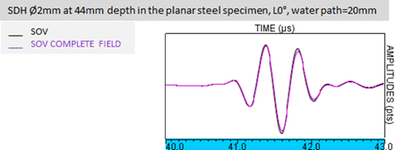
Figure 19 : Superposition of A-scans simulated with SOV and COMPLETE_SOV of the reference SDH located at 44mm depth in the steel calibration block, waterpath 20mm. It shows that both models predict simular echoes. Flat probe of Ø6.35mm, 2.25MHz.
BEAM OF THE 2.25 mhZ PROBE IN WATER
Figure 20 and Figure 21 here below show the simulated field emitted by the probe in watter.
The maximal amplitude emitted by the probe is at 15.5 mm distance form its axis. At this point, the -3dB focal spot width measures 1.9 mm and increases on each size (Figure 20).
The Ø4 and 6 mm inclusions are also much larger than the focal spot, as it can be seen on the Figure 21, where inclusions are represented with the same scale as the one of the field cartography in order to compare their dimensions to the focal spot dimensions.
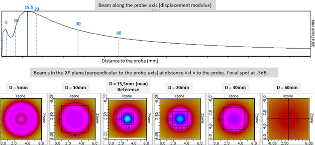
Figure 20 : CIVA simulations of the field emitted by the probe in water. On the top: field profile along the probe axis showing a maximum at a distance of 15.5 mm from the probe. On the bottom: field cartographies (6mmx6mm) in planes perpendicular to its axis at different probes distances. Comparable amplitudes (ref=maximal field amplitude obtained at D = 15.5 mm). Planar probe Ø 6.35 mm, 2.25 MHz.
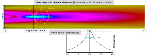
Figure 21 : CIVA simulations of the field emitted by the probe in water. Inclusions representations with the same scale as the one of the field cartography in order to compare their dimensions to the focal spot dimensions. Planar probe Ø6.35mm, 2.25MHz.
REsults obtAINED WITH STEEL INCLUSIONS
We recall in the below table the CIVA restrictions in the case of the 2.25 MHz probe that have been suppressed in order to compute the four inclusions echoes with the 3 models ; SOV, COMPLETE_SOV and SPECULAR.
|
2.25MHZ |
Inclusion Ø 1mm |
Inclusion Ø 2mm |
Inclusion Ø 4mm |
Inclusion Ø 6mm |
|
SOV |
yes |
yes |
yes |
no |
|
COMPLETE_SOV |
yes |
yes |
yes |
no |
|
SPECULAR |
no |
no |
no |
yes |
Table 2 : Avalaible models in CIVA for the computation of the inclusions echoes as a function of their diameter for the 2.25 MHz probe.
EXPERIMENTAL RESULTS
The experimental amplitude/distance echodynamic curves are presented on Figure 22. On the top, the amplitudes are relative to the reference echo amplitudes, on the bottom they are normalized:
- the maximal echo amplitude increases with the inclusion diameter. The amplitude increases by 5 to 6 dB when the inclusion diameter is doubled. It can as well be noted an increase by 3.5 dB between the 4 mm and 6 mm inclusions.
- the « dmax » distance at which the echo amplitude is maximal do practically not depend on the inclusion diameter : dmax = 14 or 14.5 mm.
- beyond « dmax », the decreasing slope do not depend on the inclusion diameter.
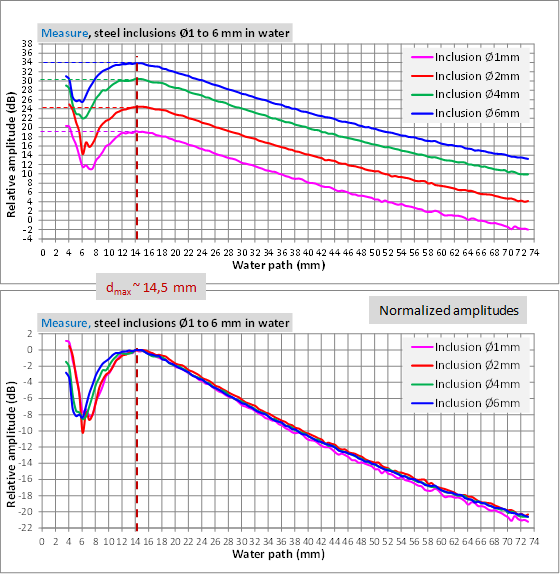
Figure 22 : Experimental results showing the evolution of the amplitude/distance echodynamic curves with the steel inclusions diameters (from 1 mm to 6 mm). On the top: comparable amplitudes, reference: L0° echo of a Ø2 mm SDH at 44 mm depth in the calibration block in ferritic steel, water path 20 mm. On the bottom: normalized amplitudes. Ø6.35 mm plane probe, 2.25 MHz.
The experimental XY curves obtained for the 4 inclusions are presented on Figure 23 (normalized amplitudes). The focal spot width does not depend on the inclusion diameter.
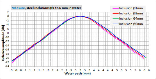
Figure 23 : Experimental results showing the evolution of the XY curves at the experimental focal distance with the steel inclusions diameters (from 1 mm to 6 mm). Normalized amplitudes. Ø6.35 mm plane probe, 2.25 MHz.
The specular echoes shape of the inclusions located at a focal distance of 14.5 mm or in the probe far field (60mm) do not depend on the inclusion diameter (Figure 24). The echo coming after the first contribution is even more far in time from the first echo than the inclusion diameter is great. The origin of the echoes appearing after the specular contribution is not accurately known, it appears a mix between the creeping waves and the waves penetratingthe inclusion in which they propagate, rebound with eventually modes conversions, interfere …
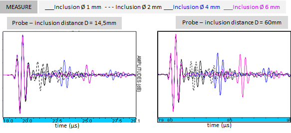
Figure 24 : Experimental results showing the A-scans evolution with steel inclusions diameters (from 1 mm to 6 mm), probe/inclusion distance = 14.5 mm on the left hand side and 60 mm on the right hand side. Normalized amplitude. Ø6.35 mm plane probe, 2.25 MHz
EXPERIMENTS/CIVA COMPARISON
-
Amplitude/distance curves
The comparisons of the measured and with SOV, COMPLETE_SOV and SPECULAR simulated amplitude/distance curves are presented Figure 25 (Ø1 mm and Ø2 mm inclusions) and Figure 26 (Ø4 mm et Ø6 mm inclusions)
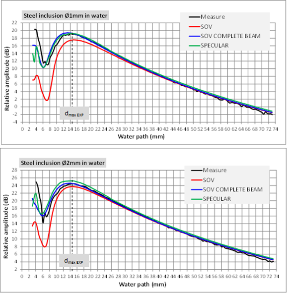
Figure 25 : Comparison of measured and with SOV, COMPLTE_SOV and SPECULAR simulated amplitude/distance curves, Ø1 mm et Ø2 mm inclusions. Reference for the amplitudes: L0° echo of a Ø2 mm SDH at 44 mm depth in a ferritic steel calibration block, 20 mm water path. In non restricted CIVA, the SOV and COMPLETE_SOV models are allowed for the Ø1 mm and Ø2 mm inclusions. Ø6.35 mm plane probe, 2.25 MHz.
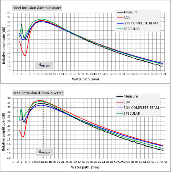
Figure 26 : Comparison of measured and with SOV, COMPLETE_SOV and SPECULAR simulated amplitude/distance curves, Ø4 mm et Ø6 mm inclusions. Reference for the amplitudes: L0° echo of a Ø2 mm SDH at 44 mm depth in a ferritic steel calibration block, 20 mm water path. In non restricted CIVA, the SOV and COMPLETE_SOV models are allowed for the Ø4 mm inclusion and the SPECULAR model is allowed for the Ø6 mm inclusion. Ø6.35 mm plane probe, 2.25 MHz.
The dmax distance at which the amplitude/distance curve amplitude is maximal is indicated in the Table 3. The differences between dmaxEXPERIMENTAL and dmaxCIVA are indicated in the table 4.
|
Distance “D” of amp max (mm) -/+0.5mm |
Simulated beam |
Inclusion Ø1mm |
Inclusion Ø2mm |
Inclusion Ø4mm |
Inclusion Ø6mm |
|
|
15.5 |
|
|
|
|
|
Measure |
|
14 |
14.5 |
14 |
14 |
|
SOV |
|
15 |
14.5 |
13.5 |
13 |
|
COMPLETE_SOV_BEAM |
|
13.5 |
14 |
13.5 |
13.5 |
|
SPECULAR |
|
14 |
14 |
13 |
14 |
Table 3: Probe/inclusion distances corresponding at the maximal amplitude of the field emitted on the probe axis or at the distances at which the amplitude/distance curve is maximal. Results of measures and with the 3 models simulations. Numbers written in bold corrispond to the non restricted cases in CIVA. Ø6.35 mm plane probe, 2.25 MHz.
|
ΔDsim/exp of amp max (mm) |
Inclusion Ø1mm |
Inclusion Ø2mm |
Inclusion Ø4mm |
Inclusion Ø6mm |
|
SOV |
1 |
0 |
-0.5 |
-1 |
|
COMPLETE_SOV_BEAM |
-0.5 |
-0.5 |
-0.5 |
-0.5 |
|
SPECULAR |
0 |
-0.5 |
-1 |
0 |
Table 4: Measures/CIVA differences between probe/inclusion distances of previous table. Numbers written in bold corrispond to the non restricted cases in CIVA. Ø6.35 mm plane probe, 2.25 MHz.
COMPLETE_SOV and SPECULAR Models : a very good agreement is obtained with the experiment for the 4 inclusions at every distances. The differences do not exceed 2 dB except for small distances. « dmax » positions are well predicted for those 4 inclusions.
More in detail:
- In far field, the measures/simulations differences are less than 1 dB for every inclusions except in the case of the Ø6 mm inclusion and of the COMPLETE_SOV model for which the measures/simualtions difference reaches a little bit more than 2 dB while SPECULAR model is closer to the measure. This gap greater than 2 dB can be attributed to a model limitation concerning the diffraction coefficient computation for the great « ka » (see here).
- Around « dmax » the amplitude/distance curves predicted by COMPLETE_SOV and SPECULAR models are in good agreement with the measure (differences of less than 2 dB).
- The deviations are more important at the very small distances but do not exceed 4 dB.
- « dmax » distance do almost not depend on the inclusion diameter according to COMPLETE_SOV and SPECULAR (Table 3) as experimentally. Both models slightly tend to underestimate « dmax » relatively to the measures, but the differences between the measured and simulated values are still less than 1 mm (Table 4).
SOV Model: the agreemnt with the measure is not so good as for the 2 previous models when the inclusions are close to the probe.
More in detail:
- In far field, the measures/simulations differences are less than 1 dB for every inclusions except in the case of the Ø6 mm inclusion for which the measures/simualtions difference reaches a little bit more than 2 dB (as with COMPLETE_SOV this gap can be attributed to a model limitation concerning the diffraction coefficient computation for the great « ka »).
- Around « dmax » the amplitude/distance curves shape predicted by SOV are not in good agreement with the measures. The gaps measures/simulations reach more than 8 dB at the distances lower than the focal distance. At the focal distance, the maximal amplitudes predicted by the SOV model are underestimated of about 2 dB for the Ø1 mm inclusion and overestimated of about 3 dB for the Ø6 mm inclusion. For the Ø2 mm and Ø4 mm inclusions, the simulated and experimental maximal amplitudes show a good agreement.
- The « dmax » distance at which the echo amplitude is maximal slightly decreases with the inclusion diameter increasing: dmax varies from 13 mm to 15 mm (Table 3) what is not in agreement with the measure. But the differences between the measures and SOV simulated values are lower than 1 dB (Table 4).
Those measures/simulations comparisons of the amplitude/distance curves point out:
- the necessity to use COMPLETE_SOV and SPECULAR rather than SOV to simulate the inclusions echoes when theu are not in far field.
- the fact that in the probe far field, the SOV and COMPLETE_SOV models give similar results.
- that the SPECULAR model predictions for the Ø6 mm inclusion in far field are closer th the measure than those obtained with the COMPLETE_SOV model for which the deviations stay low. This last observation validates the restriction that only allows SPECULAR model for the Ø6 mm inclusion in CIVA.
Simulated and experimental A-scans exemples of inclusions echoes with SOV-COMPLET and SPECULAR are rerpesented on the figure here below for both distances « D » between the probe and the inclusion. The specular echo is well predicted by SOV-COMPLET and SPECULAR. The SOV-COMPLET model also predicts quite well the contribution arriving after this echo (except for the Ø1 mm inclusion). The SPECULAR model do not simulate this contribution.
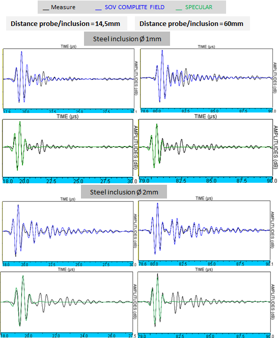
Figure 27 : Comparisons of measured and with COMPLETE_SOV and SPECULAR simulated A-scans, Ø1 mm and Ø2 mm inclusions, probe/experimental distance of 14.5 mm (experimental focal distance) and 60 mm. Non comparables normalized amplitudes. Ø6.35 mm plane probe, 2.25 MHz.
The XY experimental and with SOV, COMPLETE_SOV and SPECULAR simulated echodynamic curves, extrated at the probe/inclusion distance of 14.5 mm (experimental focal distance) as well as the -6 dB focal spot width are close (see figure here below).
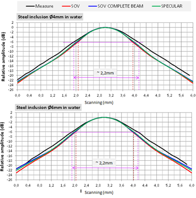
Figure 28 : Comparisons of measured and with SOV, COMPLETE_SOV and SPECULAR simulated XY curves, Ø4 mm and Ø6 mm inclusions. Normalized amplitudes. Ø6.35 mm plane probe, 2.25 MHz.
Results obtained with the infinite plan
The comparisons of the amplitude/distance curves of the infinite plane, experimental ant with SPECULAR and KIRCHHOFF models, show a very god agreement (Figure 29).
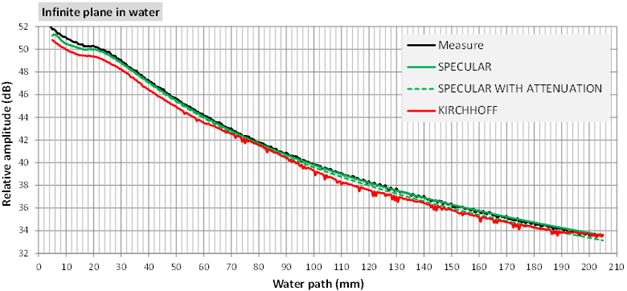
Figure 29 : Comparisons of measured and with SPECULAR (with and without attenuation) and Kirchhoff models, simulated amplitude/distance curves, infinite plane. Reference for the amplitudes: L0° echo Référence pour les amplitudes: écho L0° of a Ø2 mm SDH at 44 mm depth in a calibration block, 20 mm water path.
Ø6.35 mm plane probe, 2.25 MHz.
Note: the figure below shows that the consideration of the attenuation in water (0.0087 dB/mm at the frequency of 2 MHz) is negligible for this probe. It is recalled that for the computation of the inclusions echoes it has not been taken into account because the probe/inclusion maximal distance for the inclusions echoes measures is only 74 mm.
The experimental and with SPECULAR models predicted A-scans in the infinite plane are in very good agreement (Figure 30).
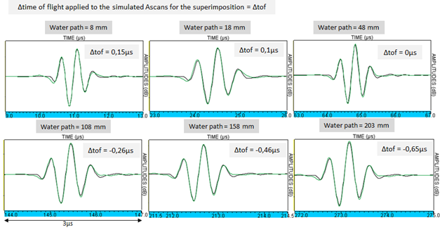
Figure 30 : Comparisons of measured and with SPECULAR simulated A-scans, infintie plane. Normalized amplitudes. Ø6.35 mm plane probe, 2.25 MHz.
ECHOES SPECTRUM OF INCLUSION AND INFINITE PLAN
Here are compared the characteristcs (central frequency « fc » and bandwidth « BW ») of measured and with SPECULAR model simulated spectra od the infinite plane at 14.5 mm (focal distance) and 60 mm (far field) in order to verify that CIVA correctly predict them. Results are gathered on the Table 5.
NB : the bandwidth indicated in MHz in the tables below is the spectrum width at the half of its maximum.
|
Infinite plane |
||||
|
Distance probe/plane |
14.5mm |
60mm |
||
|
|
fc (MHz) |
BW (MHz) |
fc (MHz) |
BW (MHz) |
|
Measure |
2 |
1.2 |
2.2 |
1.25 |
|
SPECULAR |
2 |
1.25 |
2.15 |
1.25 |
Tableau 5 : Comparisons of characteristics from measurement and with SOV, COMPLETE_SOVand SPECULAR simulated results (central frequency fc and bandwidth BW) of the specular echoes spectrum of the infinite plane in water at 14.5 mm and 60 mm from the probe. The values written in bold correspond to the non restricted cases in CIVA.
Ø6.35 mm plane probe, 2.25 MHz.
The same extracted experimental and simulated characteristics of inclusions echoes spectra have been compared with the characterictics from the infinite plane. The Table 6 shows an example of Ø1mm inclusion results.
|
Inclusion Ø1mm |
||||
|
Distance probe/inclusion |
14.5mm |
60mm |
||
|
|
fc (MHz |
BW (MHz) |
fc (MHz) |
BW (MHz) |
|
Measure |
2 |
1.2 |
2.1 |
1.2 |
|
SOV |
2 |
1.1 |
2.1 |
1.1 |
|
SOV-COMPLETE-BEAM |
1.9 |
1 |
2.1 |
1.05 |
|
SPECULAR |
1.9 |
1.1 |
2.1 |
1.3 |
Tableau 6 : Comparisons of characteristics from measurement and with SOV, COMPLETE_SOV and SPECULAR simulated results (central frequency fc and bandwidth BW) of the specular echoes spectrum of the Ø1mm steel inclusion in water at 14.5 mm and 200 mm from the probe. The values written in bold correspond to the non restricted cases in CIVA.
Ø6.35 mm plane probe, 2.25 MHz.
Those results show that CIVA correctly predicts the central frequencies and bandwidths of the echoes of the infinite planes in both inclusions. The values do almost no depend on the reflector.
EFFECT OF small CHANGEs IN the central frequency
It has been evaluated the effect of an arbitrary variation of +/-0.1 MHz of the centrale frequency « fc » of the entry signal (almost 5 % of the probe nominal central frequency) on the CIVA predictions for the inclusions and the infinite plane.
Before studying this effect on the inclusions echoes and infinite plane, the experimental/simulated good agreement for the SDH reference echo for the three evaluated frequencies (2.2 MHz, 2.3 MHz and 2.4 MHz) has been verified because it is essential to allow the measure/simulation comparisons for other reflectors.
The reference echo A-scans (SDH) simulated at the three frequencies are in agreement with the measure (Figure 31).
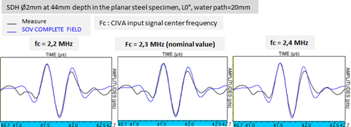
Figure 31 : Superimposition of the measured and with COMPLETE_SOV simulated A-scans of the reference SDH echo. Those comparisons show that the with COMPLETE_SOV simulated A-scans for central frequencies of 2.2, 2.3 and 2.4 MHz are all in good agreement with the measure. Normalized amplitudes. Ø6.35 mm plane probe, 2.25 MHz.
In the same way, the reference SDH amplitude (at 44 mm depth) varies a little bit with the central frequency: almost 0.5 dB (Figure 32).
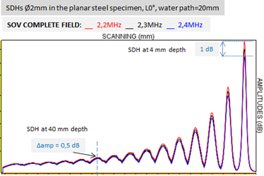
Figure 32 : COMPLETE_SOV simulation results, SDH L0° echoes at different depth (from 4 mm to 60 mm by 4 mm steps) in the calibration block. Study of the effect of a low central frequency variation on this curve calculated for three frequencies: 2.2 MHz, 2.3 MHz and 2.4 MHz. Ø6.35 mm plane probe, 2.25 MHz.
The inclusions ampitude/distance curves has been simulated at the 3 central frequencies « fc » with the COMPLETE_SOV models for the Ø1, 2 et 4 mm inclusions (Figure 33) and SPECULAR model for the Ø6 mm inclusion (Figure 34).
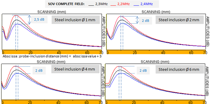
Figure 33 : COMPLETE_SOV simulation results, amplitude/distance curves of steel inclusions in water. Study of the effect of a low variation of the central frequency on the curves obtained for 3 frequencies: 2.2 MHz, 2.3 MHz and 2.4 MHz. Ø6.35 mm plane probe, 2.25 MHz.
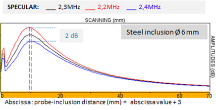
Figure 34 : COMPLETE_SOV simulation results, amplitude/distance curves of the Ø6mm steel inclusion in water. Study of the effect of a low variation of the central frequency on this curve obtained for 3 frequencies: 2.2 MHz, 2.3 MHz and 2.4 MHz. Ø6.35 mm plane probe, 2.25 MHz.
Those results show the a probe central frequency variation modifies the maximal amplitude of the amplitude/distance curves by 2 dB to 2.5 dB. However, when the inclusions move away from the probe, the amplitudes of their echoes vary a little with fc.
Also, if the CIVA entry signal central frequency is modified by 0.1 MHz, the maximal amplitudes of the inclusions amplitude/distance curves can vary by almost 2 dB if the reference for the amplitudes is the SDH at 44 mm depth. Moreover, the amplitude/distance curve maximal position varies by 1.5 mm. Those variations can be considered as uncertainties on CIVA simulation results related to the value uncertainty of the entry signal of the central frequency.
Synthesis
A very good agreement has been obtained for this probe between the measures and with COMPLETE_SOV and SPECULAR simulations for:
- the amplitude/distance curves and the inclusions and the infinite plane,
- the « XY » curves and the inclusions,
- the echoes A-scans and their spectra.
The overestimation of the Ø6 mm inclusions echoes amplitude in far field with SOV and COMPLETE_SOV justify the current restriction in CIVA which only allow echoes computation of this inclusion with SPECULAR model. The COMPLETE_SOV contribution related to SOV has been pointed out for the inclusions echoes when they are close to the probe.
Continue to Results obtained with the 5 MHz probe
Back to Simulation settings
Back to Single element probe