
UT – Phased Arrays – Experimental and simulation set-up
Summary
EQUIPMENT and confidence interval of experimental data
Experimental acquisitions were performed with an equipment composed of a mechanical bench allowing C-scan and an electronic phased array acquisition system MultiX 64 controlled with the Multi2000 V6.5.22 software. An inspection procedure was followed to minimize sources of uncertainty. The global uncertainties associated with mechanical parameters, machined defects, and material homogeneity was assessed by verifying the reproducibility of the results. The confidence interval of the experimental data has been estimated to be +/-3 dB for contact probes (1.5 dB due to the uncertainty of the measurement on the calibration defect and 1.5 dB due to the uncertainty of the measurement relatively to the reference) and +/-2 dB for immersion probes (1 dB due to the uncertainty of the measurement on the calibration defect and 1 dB due to the uncertainty of the measurement relatively to the reference).
Specimens
Two ferritic steel specimens (cL=5900 m/s, cT=3230 m/s, density = 7.8 g/cm3) are inspected:
- A mock-up containing a set of Side-Drilled Holes (SDHs) of diameter Ø2 mm and 60 mm long. They are located at depths from 4 mm to 60 mm with 4 mm step between each defect.
Ø2 mm diameter SDH (extension 60 mm) specimen
- A mock-up containing sets of Flat Bottom Holes (FBHs) of diameter 1 mm, 3 mm and 6 mm and tilted at 45°.
FBHs of a specific diameter are located at two different increments in order to avoid echoes mixing during inspection. The depths corresponding to the first increment are 5 mm, 15 mm, 25 mm, 35 mm, 45 mm, 55 mm, 80 mm, 100 mm, 125 mm and 150 mm. The depths corresponding to the second increment are 10 mm, 20 mm, 30 mm, 40 mm, 50 mm, 60 mm.

Specimen with FBH of 1 mm, 3 mm et 6 mm diameter and tilted with 45°
Probes
Measurements were performed with three probes:
2 MHz matrix contact probe
The technical characteristics of this probe are listed in the table below:
| Type | Pattern | Number of elements | Pitch | Frequency | Bandwitch | Phase |
| Contact | Matrix | 64 (16×4) | 0.2 mm (raw and column) | 2 MHz | 60% | 65° |
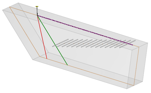
This probe is fixed to a rexolite wedge (cL=2320 m/s). The wedge incidence angle is 16.86° which corresponds to a refraction angle of 47.5° in ferritic steel for longitudinal waves. These parameters were determined from the wedge backwall echo. This method consists in performing an electronic scanning of 1 active element and to register the wedge backwall echo relatively to the active sequence. The time propagation of the wedge backwall echo (between the edges elements 3 and 63), the knowledge of the distance between these two elements and the wave velocity in the wedge allow to determine the wedge angle.
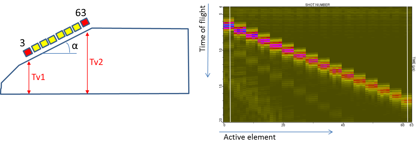
Method for wedge incidence angle measurement
Field calculations allow to find the near field limit of the probe. The following figure shows the P transmitted field. It can be seen that beyond 30 mm, the probe does not focus at the desired depth. The near field limit for P waves is close to 30 mm.
Civa simulation results, refracted P beams in the specimen, in the inspection plane, displacement module
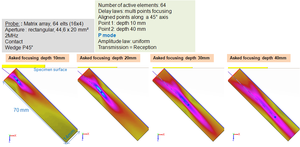
For SV waves, field calculations provide the following results:
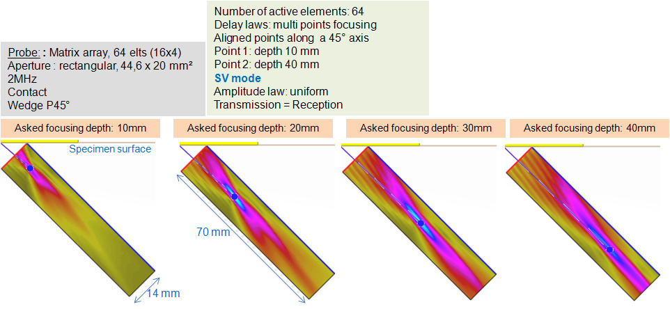
Civa simulation results, refracted SV beams in the specimen, in the inspection plane, displacement module
This figure shows that the near field for SV waves is around 40 mm depth.
5 MHz linear contact probe
The technical characteristics of this probe are listed in the table below:
| Type | Pattern | Number of elements | Pitch | Frequency | Bandwitch | Phase |
| Contact | Linear | 48 | 0.1 mm | 5 MHz | 64% | 20° |
This probe is fixed to a rexolite wedge (cL=2320 m/s). The wedge incidence angle is 21° which corresponds to a refraction angle of 65.7° in ferritic steel. The wedge characteristics were obtained with the same method as for the 2 MHz probe.
Three parameters have to be precised in CIVA for the attenuation law in SV mode: the attenuation coefficient “a”, the attenuation law exponent and the frequency “f “:
- The chosen frequency “f” corresponds to the central frequency of the signal transmitted by the probe (4.8 MHz)
- In the studied specimens, the attenuation coefficient was found during a previous study that showed that it is not necessary to take into account attenuation for P waves. For SV waves, with an exponent of 4 (Rayleigh domain), a = 0.015 dB/mm.
Field calculations in P wave allow to determine the near field limit of this probe. It can be seen on the figure below that beyond 20 mm depth, the probe does not focus accurately. It is then the probe near field limit in P wave.
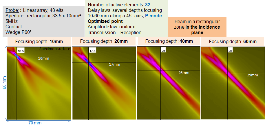
Civa simulation results, refracted P beams in the specimen, in the inspection plane, displacement module
For SV waves, field calculations provide the following results:
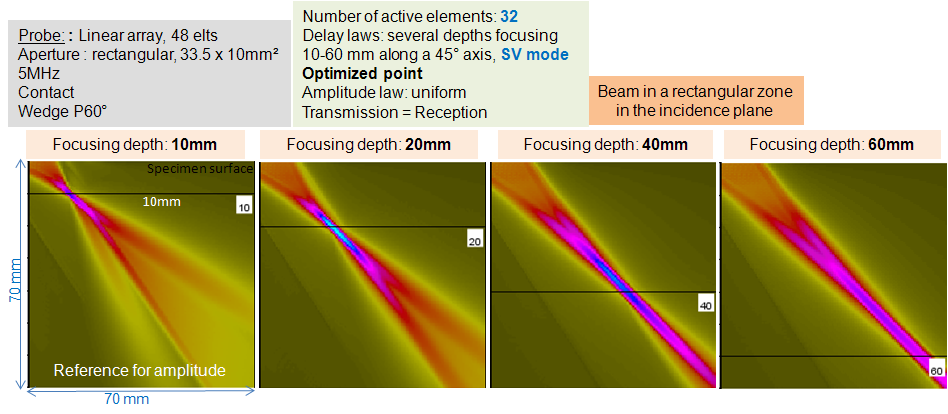
Civa simulation results, refracted SW beams in the specimen, in the inspection plane, displacement module
These results show that the near field limit for SV wave is 40 mm.
10 MHz immersion probe
The technical characteristics of this probe are listed in the table below:
| Type | Pattern | Number of elements | Pitch | Frequency | Bandwitch | Phase |
| Immersion | Linear | 32 | 0.05 mm | 10 MHz | 55% | 290° |
Attenuation law for P waves
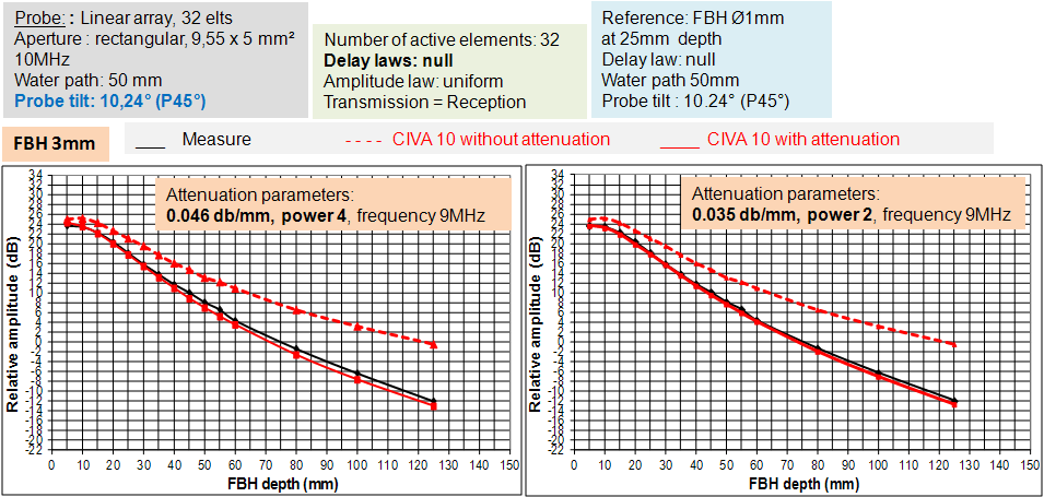
The P waves attenuation law was determined from the FBHs echoes obtained with a probe tilted a 10.24° angle (P45°), a water path of 50 mm and a null delay law.
Parameters to enter in CIVA (attenuation coefficient “a”, attenuation law exponent and the frequency “f”):
- The frequency “f” is the central frequency of the transmitted signal (9 MHz)
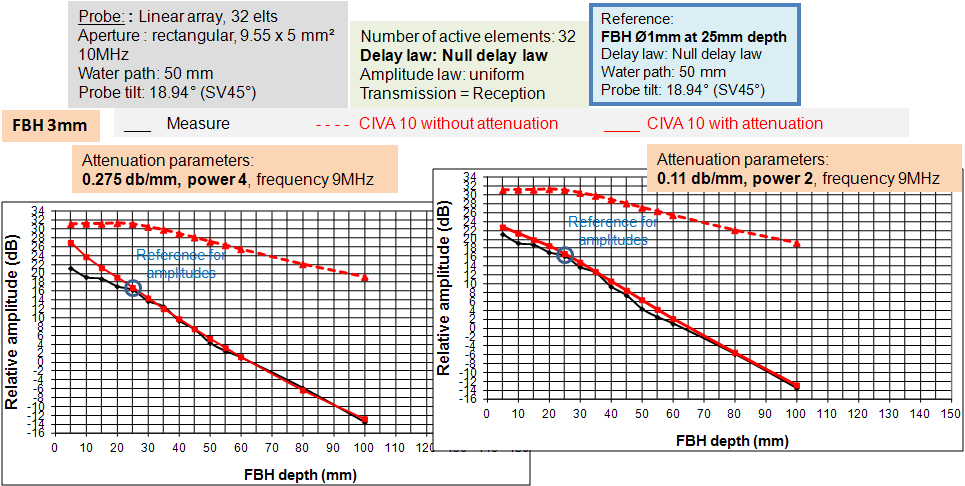
- Two attenuation coefficients were determined by adjusting their value so that experimental and simulated amplitude curves of P direct echoes of FBH Ø3 mm present the same decreasing. These adjustments were performed on the curves resulting from a null delay law.
The reference amplitude is the one of a FBH Ø1 mm located at 25 mm depth. The reference amplitude was also simulated with attenuation:
- The first coefficient was determined for an exponent of 4 (Rayleigh domain : λ >> D), in this case a = 0.046 dB/mm
- The second was determined for an exponent of 2 (stochastic field : λ ~ D), in this case a = 0.035 dB/mm
With λ the wavelength and D the mean grain size constituting the microstructure.
In the following, the first attenuation law will be called (0.046, 4, 9) or law in exponent “4” and the second one (0.035, 2, 9) or law in exponent “2”.
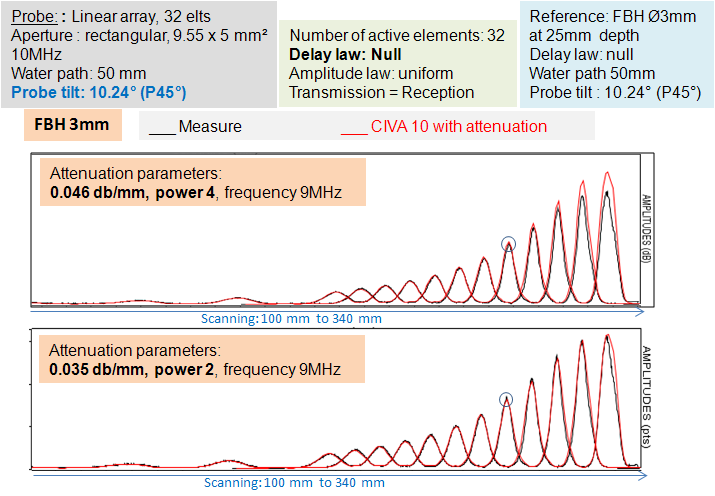
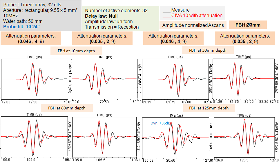
Ø3 mm FBH amplitude comparison , echodynamic curves comparison and Ascan comparison (experiment / CIVA)
It can be seen on the figure above that there is a good agreement between experimental and simulated Ascans for FBHs located at small depths. This is no more the case for deeper defects when applying the attenuation law (0.046, 4, 9) ; the simulated Ascans are then too “low frequency” compared to the experimental Ascans. With the law in exponent “2”, (0.035, 2, 9), there is a better agreement between simulation and experiments for deep FBHs (80 mm and 125 mm). These comments are also available for FBHs of 1 mm and 6 mm diameter.
According to these results, the attenuation law in exponent “2” will be used for simulations. The law in exponent “4” can be used to validate this choice.
Attenuation law for SV waves
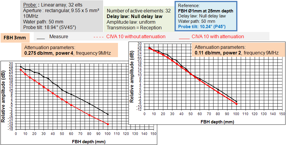
The SV waves attenuation law was determined from FBHs echoes obtained with a probe tilted with a 18.94° angle (SV45°), a water path of 50 mm and a null delay law.
Parameters to enter in CIVA (attenuation coefficient “a”, attenuation law “exponent” and the frequency “f”):
- The frequency “f” is the central frequency of the transmitted signal (9 MHz)
- The two attenuation coefficients were determined by adjusting their value so that experimental and simulated amplitude curves of SV direct echoes of FBH Ø3 mm present the same decreasing. These adjustments were performed on the curves resulting from a null delay law.
The reference amplitude is the one of a FBH Ø1 mm located at 25 mm depth. The reference amplitude was also simulated with attenuation:
- The first coefficient was determined for an exponent of 4 (Rayleigh domain : λ >> D), in this case a = 0.275 dB/mm
- The second was determined for an exponent of 2 (stochastic field : λ ~ D), in this case a = 0.11 dB/mm
With λ the wavelength and D the mean grain size constituting the microstructure
In the following, the first attenuation law will be called (0.275, 4, 9) or law in exponent “4” and the second one (0.11, 2 9) or law in exponent “2”.
Ø3 mm FBH echoes amplitude comparison (experiments/CIVA) in SV mode, amplitude reference is the one measured on the SV echo of a Ø1 mm FBH located at 25 mm depth
If the amplitude reference is the one from a P direct echo of FBH, the SV echoes amplitudes simulated with the attenuation law (0.275, 4, 9) are very different from experimental ones (cf. figure below).
Ø3 mm FBH echoes amplitude comparison (experiments/CIVA) in SV mode, amplitude reference is the one measured on the P echo of a Ø1 mm FBH located at 25 mm depth
As for P waves echoes, it can be seen on the figure below a good agreement between experimental and simulated Ascans for FBHs located at small depths. It is not the case for deeper defects when applying the attenuation law (0.275, 4, 9) ; the simulated Ascans are then too “low frequency” compared to the experimental Ascans. With the law in exponent “2”, (0.11, 2, 9), there is a better agreement between simulation and experiments for deep FBHs (80 mm and 125 mm). These comments are also available for FBHs of 1 mm and 6 mm diameter.
According to these results, the attenuation law with exponent “2” will be used for simulations. The law in exponent “4” can be used to validate this choice.
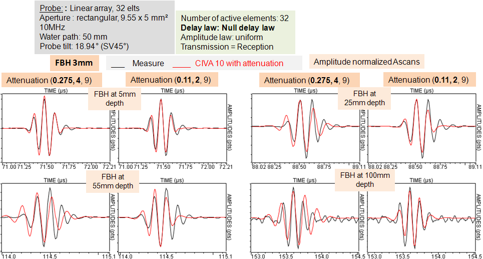
Ascans comparison for FBH Ø3 mm located at different depths, SV direct mode
Field calculation in P wave (see figure below) shows that beyond 10 mm depth, the probe does not focus accurately. The near field limit is then 10 mm.
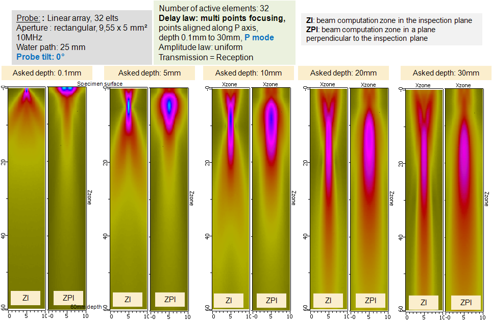
CIVA simulation results, P transmitted field in the specimen, in the inspection plane
INTERACTION models
Models defined in CIVA to simulate responses defects are:
- The SOV model (Separation Of Variables) for SDHs
- The Kirchhoff model for FBHs
Continue to Results obtained with the several depths focusing algorithm
Back to Phased arrays