
Shadowing – Experimental and simulation setups
Summary
Specimen and experimental measurements
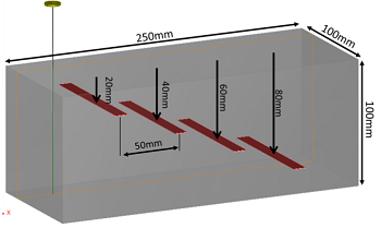
A specific mock-up has been realized for this study. It is a flat steel specimen of 100 thickness containing ribbons-like defects (they will be called ribbons in the following) parallel to the surface and located at 20mm, 40mm, 60mm, and 80mm, depth. These ribbons of 10mm length are passing through the 100m wide specimen.
Probes
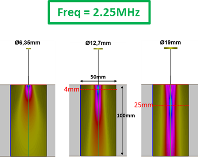
The acquisitions were performed with planar circular immersion single element probes of 3 different apertures (Ø6.35, 12.7 and 19mm) and of central frequency 2.25MHz and 5MHz. They have null incidence angle in order to generate L0° waves in the component. The ultrasonic beams associated with these 3 apertures, for 50mm water path, are displayed below for 2.25 MHz and 5 MHz.
Experimental acquisitions were performed with equipment composed of a mechanical bench allowing C-scan acquisition and an electronic phased array acquisition system MultiX 64 controlled with the Multi2000 V6.7.32 software. An inspection procedure was followed to minimize sources of uncertainty. The global uncertainties associated with mechanical parameters, machined defects, and material homogeneity was assessed by verifying the reproducibility of the results. The experimental data interval of confidence has been estimated to be +/-2 dB (1dB due to the uncertainty of the measurement on the calibration defect and 1 dB due to the uncertainty of the measurement relatively to the reference).
Compared echoes
The maximum amplitudes of the ribbons specular echoes and the backwall echoes amplitudes with or without shadowing are measured. The experimental and simulated amplitudes are then compared.
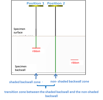
Two probe positions relatively to a ribbon are defined (figure below):
- Position 1: the probe axis is located at the ribbon center; this corresponds to a probe position where the backwall is shadowed by the defect. In the following, this backwall area will be called “shadowed backwall zone”
- Position 2: the probe axis is equidistant from the edges of 2 ribbons. This corresponds to a position where the backwall is not shadowed by a defect. In the following, this area will be called “non- shadowed backwall zone”.
The zone between these 2 positions is called “transition zone between the shadowed backwall and the non-shadowed backwall”.
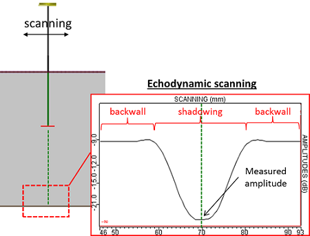
The figure below shows an example of an echodynamic curve obtained when the probe is located around position 1. In the following, the amplitude measured at this position will be called “ribbon shadowed backwall echo amplitude”.
The Ascans and the experimental and simulated echodynamic curves are also compared.
Calibration amplitude
The calibration amplitude is the maximal amplitude measured on a L0° SDH (Ø2mm) direct echo. The SDH is located in a calibration specimen made of the similar steel than the shadowing specimen described previously. The SDH depth corresponding to the maximal amplitude according to the probe aperture is:
| Ø19 mm | Ø12.7 mm | Ø6.5 mm | |
| 2.25 MHz | Ø2 mm SDH at 24 mm depth | Ø2 mm SDH at 8 mm depth | Ø2 mm SDH at 10 mm depth |
| 5 MHz | Ø2 mm SDH at 60 mm depth | Ø2 mm SDH at 25 mm depth | Ø2 mm SDH at 5 mm depth |
Simulation parameters
The simulations were performed with CIVA 11.0a:
- CIVA (beam simulations and defect responses were performed with CIVA11.0a and the « 3D » calculation options); the defect responses are realized with KIRCHHOFF+GTD model for the ribbons and with the SOV model for the SDH. The backwall echo calculation was performed with 2 models: the Kirchhoff model and the Specular model. The results of both models are compared in the following.
- ATHENA2D (« 2D » Finite Element modeling for the defect interaction coupled with the CIVA 11.0a beam calculation performed with the « 2D » option.)
The CIVA input parameters are reported below:
« Shadowing » specimen material :
| L wave velocity | T wave velocity | density | attenuation |
| 5950 m.s-1 | 3290 m.s-1 | 7.8 g.cm-3 |
|
The L and T wave velocities were obtained by experimental measurements of successive backwall echoes times of flight in the flat specimen of 100mm thickness. A 5MHz L0° probe was used for L wave velocity measurement whereas a 5MHz T0° probe was used for T wave velocity measurements.
Calculation precisions for beam and echoes simulations: 3 and 3.
Justification of the need to calculate additional modes in addition to the direct mode
Direct mode only
The figure below shows simulation results obtained in direct L mode with the 2.25 MHz probe of Ø19mm diameter and with the 2 backwall echo calculation models available in CIVA ( KIRCHHOFF and SPECULAR).
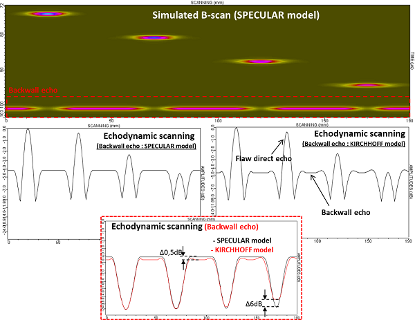
The results of the shadowed and non-shadowed backwall echo with the 2 models show some differences:
- There is an increase of the amplitude with the KIRCHHOFF model in the transition zone between the shadowed backwall and the non-shadowed backwall. This is not the case with the SPECULAR model.
- For the deeper flaw (80 mm depth), the shadowed backwall echo zone amplitude is 6dB stronger with KIRCHHOFF than with the SPECULAR model.
Mode taking into account a skip on the backwall before or after interaction with the flaw
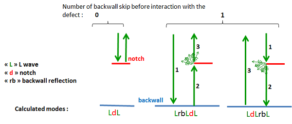
CIVA simulations, taking into account both L direct mode and the one with a skip on the backwall before interaction with the defect, were performed. The figure below shows the calculated ultrasonic paths and the calculated modes in function of the number of skips on the backwall.
The echodynamic curves obtained with the KIRCHHOFF and the SPECULAR models are presented on the figure below. The black curves represent the result when only the direct mode is calculated while the red curves take into account a skip on the backwall. In the latter case, the backwall and the defect echoes associated with the skip are mixed.
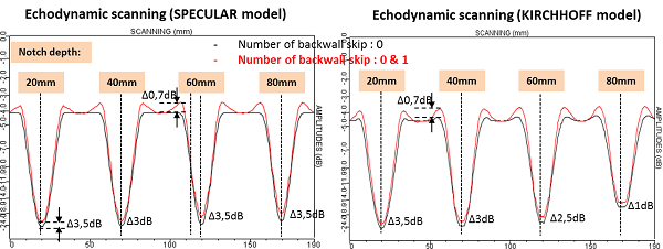
These results show that when a skip on the backwall is taken into account before interaction with the flaw:
- An increase of the amplitude in the transition zone between the shadowed and non-shadowed backwall for both models is observed. This increase is equal to 0.7dB relatively to the direct mode and is due to the diffraction echo of the ribbon edges after skip on the backwall (second figure above).
- When the probe is located above the ribbon, a change on the backwall amplitude echo is observed. Simulation results highlight weaker shadowing when the skip on the backwall is taken into account. The amplitude difference may reach 3.5 dB. When using KIRCHHOFF, the difference may be bigger as the defect is far from the backwall. Indeed, +3.5dB have been measured for the 20mm depth ribbon while +1dB for the 80mm depth ribbon.
Thus, the next presented simulations were performed with 1 backwall skip taken into account. The beam interaction with the backwall is calculated with the 2 models available in CIVA11: SPECULAR and KIRCHHOFF. The beam interaction with the flaw is performed with the KIRCHHOFF+GTD model.
Continue to Results with the Ø19mm single element probe
Back to Shadowing