
Calibration: The input signal in CIVA
Summary
In the Civa “Defect Response” module, the input signal theoretically corresponds to the second time derivative of the acoustic particle velocity normal to the crystal surface (detailed information explaining this relation can be asked to the support team at supportciva[at]extende.com).
But, as this acoustic particle velocity is not easy to determine, we propose below simple ways to obtain this input signal.
In CIVA, the input signal can either be loaded from an external text file (obtained from a measured calibration echo) or defined in CIVA as a “synthetic” signal (defined with parameters assuming a Hanning or a Gaussian frequency distribution).
- In the case of a synthetic input signal, the centre frequency, bandwidth and phase of the input signal have to be determine by the user, and we will propose detailed methods for their determination.
- In the case of an experimental input signal (external text file), we will explain which calibration flaws are used to measure the calibration echo.
This will be illustrated on an example: the determination of the input signal for a SV45° inspection performed with an immersion probe (planar, Ø6.35 mm, 2.24 MHz, water path 25 mm).
Practical information about input signal
To access the input signal in Civa, you have to open the “Signal” tab from the “Probe” panel.
- If only manufacturer data are available or if a synthetic signal is going to be used as input signal, you click on the “edit” button and a new window appears where you can define the waveform, the phase and the sampling of the input signal.
- If a specular echo from a reference flaw is stored as a text file, it should be loaded by clicking on the “load” button.
Synthetic input signal
The aim of this section is to answer this question:
How to determine the centre frequency, bandwidth and phase of the input signal?
Two method will be explained for the frequency and the bandwidth. Then some information will be given about the phase and the sampling of the input signal:
- First method: from data provided by the probes manufacturer
- Second method: from the experimental echo of a calibration flaw
- How to determine the phase of the input signal?
- Practical information about the sampling of the input signal
First method: from data provided by the probes manufacturer
If available, the probe parameters from the manufacturers (centre frequency (fc), bandwith (BW)) are often sufficient to define a reference signal in terms of waveform. The phase, in this case, is put to 0° for example.
Second method: from the experimental echo of a calibration flaw
The central frequency and bandwidth of the input signal can be directly deduced from the experimental echo of a calibration flaw. In our example, this experimental echo is the specular echo of a Ø2mm Side Drilled hole (SDH) positioned at 4mm depth. The Fscan of this echo is used to determine the central frequency and bandwidth of the input signal:
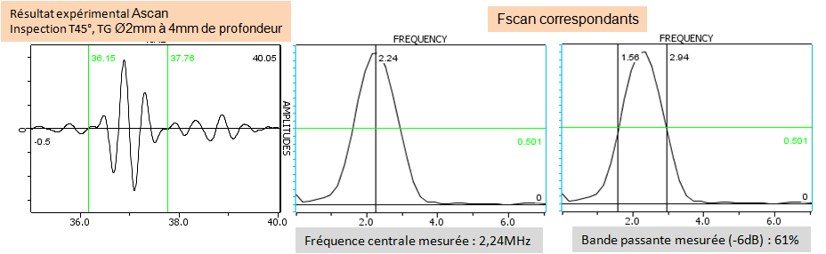
The central frequency of the input signal is 2.24 MHz. The bandwidth of the input signal is 61%.
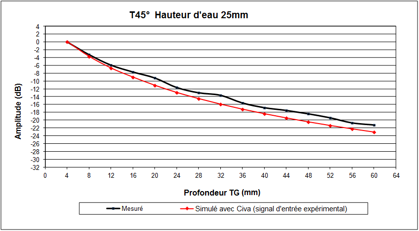
As we can see on the next figure, the measured and Civa simulated amplitudes of SDH at different depths are in good agreement (discrepancies of less than 2 dB).
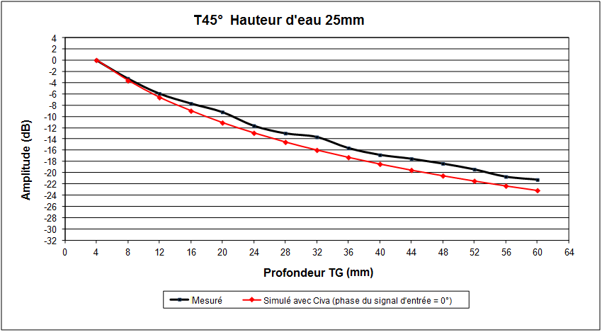
Input signal: fc=2.24MHz, BW=61% and phase=0°.
How to determine the phase of the input signal?
The inspection often requires only the envelop of the input signal. But if the phase is necessary to enable the comparison between the experimental and simulated Ascans, it can be adjusted: the procedure consists in adjusting the phase parameter of the input signal in order to reproduce after simulation of the reference flaw inspection the same signal as the experimental echo from the reference flaw.
For further information of the phase obtained after simulation on a SDH or a FBH, you could contact the support team at supportciva[at]extende.com.
In our example, the reference flaw is a Ø2 mm Side Drilled hole (SDH) positioned at 4 mm depth. We calculated with Civa the echoes of this reference SDH with different input signals having the previously determined centre frequency (2.24MHz) and bandwidth (61%) but having various phases (0°, 280°, 300° and 320°, see figures below). We compare the different simulated Ascans obtained with the experimental one (figure below).
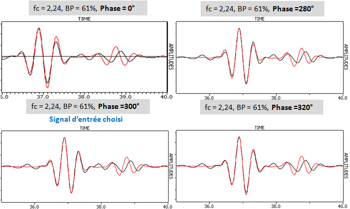
We can see that the simulated Ascan obtained with the phase 300° is very close to the experimental one: this value of 300° will be chosen for the input signal.
As we can see on the next figure, with this input signal (fc=2.24 MHz, BW=61% and phase=300°), the measured and Civa simulated amplitudes of SDH at different depths are still in good agreement (as previously said and noticed by comparing figures corresponding to different phases, the phase of the input signal doesn’t have a strong effect on the Ø2mm SDH echo amplitudes, the phase adjustment is useful to compare measured and simulated Ascans).
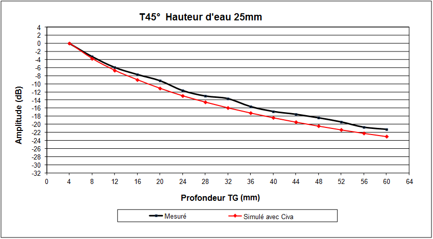
Input signal: fc=2.24MHz, BW=61% and phase=300°
Practical information about the sampling of the input signal
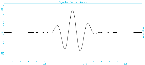
The input signal has to be digitized. The sampling frequency of the input signal should be at least 25 times its central frequency. The number of points just needs to be large enough so that the signal at starting and ending times is close to zero, as in the following image.
EXPeRIMENTAL input signal
In Civa “Defect Response” module, as previously said, the input signal is supposed to be the second time derivative of the acoustic particle velocity. It can be shown (contact the support team at supportciva[at]extende.com for additional information) that in most inspection cases the correct input signal can be deduced in a good approximation from the echo measured on a calibration reflector.
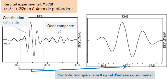
In our example, we choose as an experimental input signal, the specular echo of a Ø2mm Side Drilled hole (SDH) positioned at 4mm depth. This specular echo is represented on the next figure (only the specular contribution of the echo is used as input signal, the creeping wave contribution has to be eliminated):
As we can see on the next figure, with this experimental input signal, the measured and Civa simulated amplitudes of SDH at different depths are still in good agreement.
Experimental input signal (SDH Ø2 mm at 4 mm depth echo)
Continue to The reference amplitude
Back to Calibration