Thermographic Testing with CIVA
CIVA TT covers two applications:
- “Optical Thermographic Inspection Simulation“: This tool provides thermograms versus time
- “Induction Heating computation“: This tool provides power density maps induced by an inductor
Through simulation in CIVA, you can easily compare a large variety of optical heating techniques (Flash, Transient, Lock-In, etc.) to improve inspection regarding many scenarios, maximize temperature contrasts and defect detectability. Change specimen and flaw characteristics, modify environment properties, define your thermographic inspection technique, and repeat these steps to generate thermal images and data.
CIVA TT allows you to evaluate the impact of specific thermal parameters related to the environment (such as emissivity and environment temperatures) and to the technique (detector position in reflection or transmission mode, excitation type, power and heating time). Study the reliability of your thermographic inspection regarding various specimens and flaws (geometry type and dimensions, positions and orientations, materials). Perform parametric studies to focus on the influence of one parameter or a combination of several ones.
To manage efficient parametric studies, this module is also compatible with the following CIVA features: Parametric Study, Metamodels and CIVA Script.
Simulations examples
Specimen
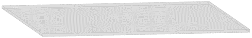
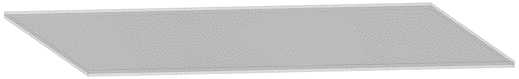
Metallic or composite plate, possibly multi layers are available in CIVA TT Inspection Simulation:
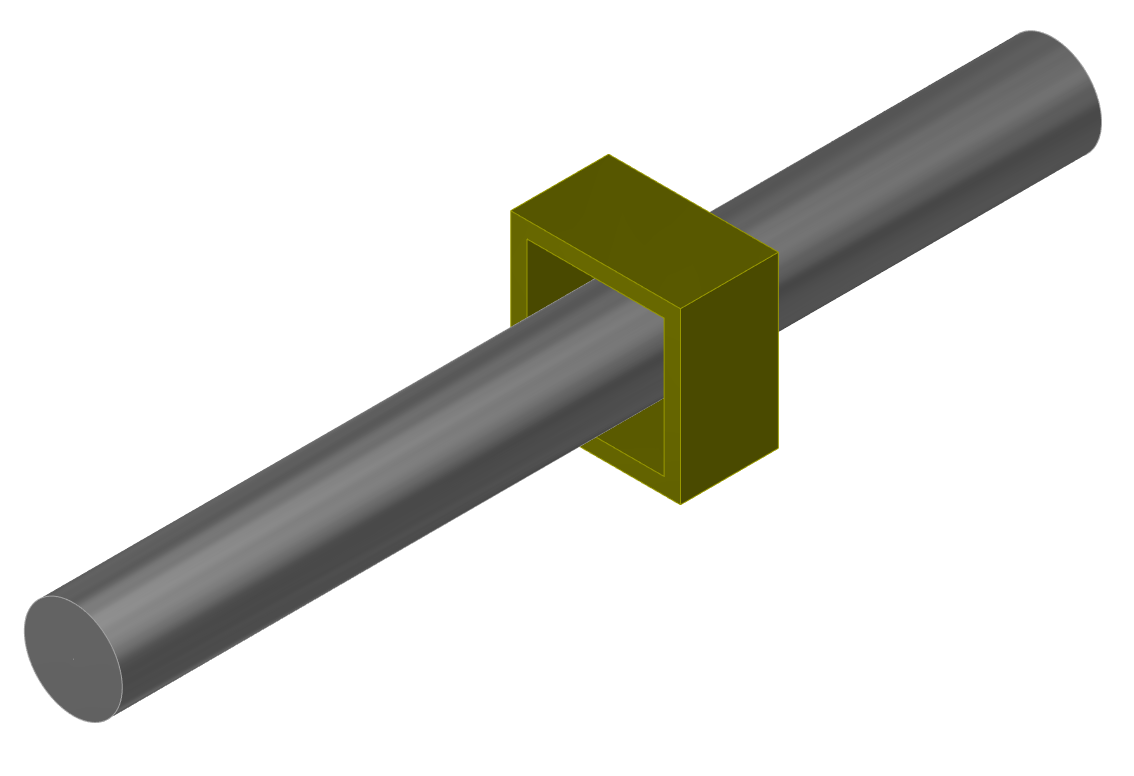
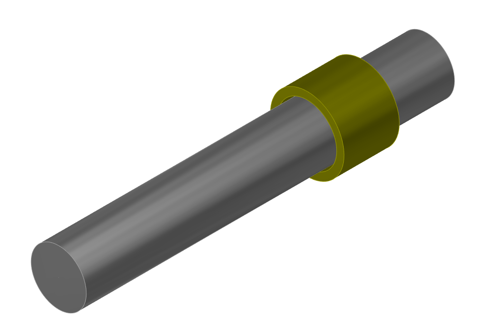
The following geometries are available in the Induction Heating module (conductive materials):
- Planar, possibly multi layers
- Cylindrical
- 2D CAD
- Fastened Plate
- Expanded Tube
- Blade Root
- Blade Groove
- Weld (T or Butt Weld)
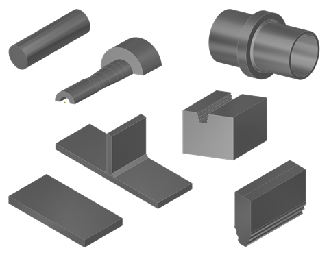
Examples of geometries taken into account by CIVA TT Induction Heating Computation
Materials are assumed to be isotropic with linear properties. Inspection Simulation module requires the definition of thermal properties (thermal conductivity and Volumetric Heat Capacity) while the Induction Heating module needs the definition of electromagnetic properties (electrical conductivity, relative permeability).
A database of several materials is provided.
Inductor
Several inductor types can be defined in the Induction Heating module, a simple air-core cylindrical coil, or with a ferrite core, other coil shapes such as rectangular ones, that can be mounted around a U-Yoke. A sinusoidal current source is defined and several channels operating at different frequencies can be considered in the same model.
Source
Various types of Optical Heating lamps can be defined in the Inspection Simulation module. Five excitation models can be selected:
- Impulse source, representative of Flash lamps
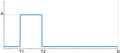
- Crenel source, representative of Halogen Lamps (Transient Thermography)
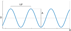
- Sinusoidal source, representative of Lock-in technique
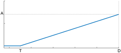
- Ramp
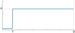
- Step
The lamp is assumed to heat uniformly the top surface of the component.
Detector
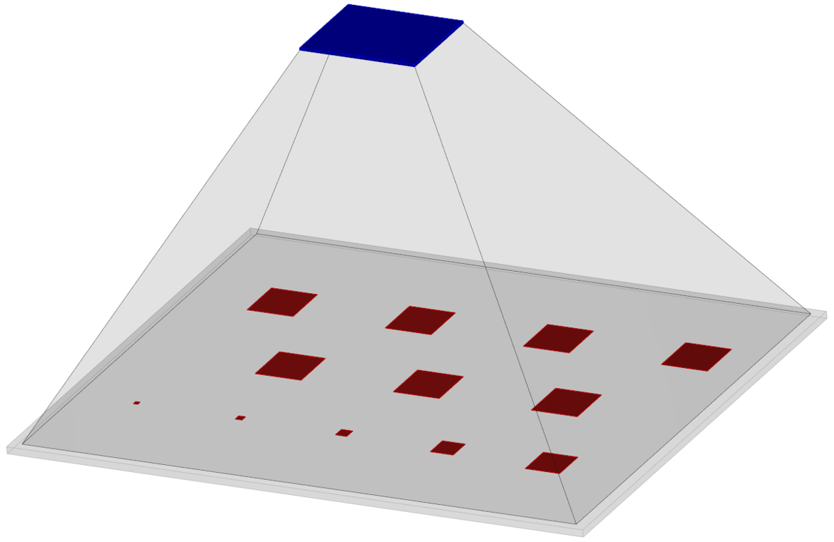
The IR camera is modelled by a rectangular detector that can be positioned on the same side of the source, reflection technique, or on the opposite one for the transmission technique.
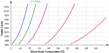
The detector resolution is parametrized by the pixel sizes and the focal distance. The camera response is modelled by a transfer function converting specimen temperature to digital levels.
Three detectors models are proposed:
- Perfect detector
- Calibration curve definition
- Equation
Some noise can be considered on the detector. The camera response is also affected by environmental properties and temperature (atmosphere and surrounding objects) as well as the emissivity of the specimen.
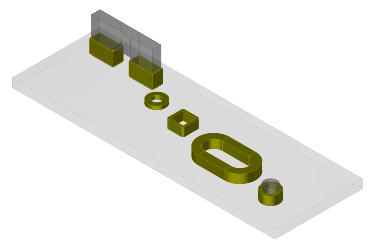
Flaws
3 defect geometries can be defined in the Inspection Simulation module:
- Planar geometry: To model crack-like defects, delamination, Teflon inserts or parallelepiped solid inclusions
- Cylindrical geometry: To model Side Drilled Holes or cylindrical inclusions
- 2.5D CAD geometry: To model volumetric wall thickness loss or inclusion of arbitrary section
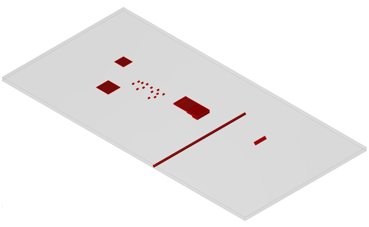
Types of defects available in CIVA TT
Results
Inspection Simulation
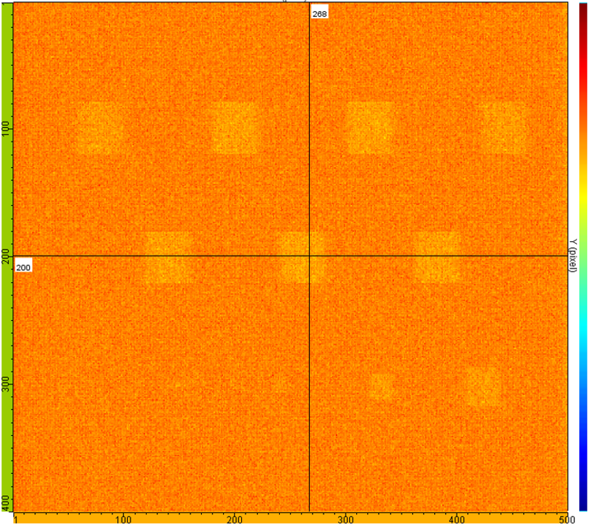
The Inspection Simulation module computes the thermal heating process versus time by solving the Fourier Heat Law with a very fast 2D Finite Integration Technique solver. It gives the digital levels obtained on the IR camera accounting for the heating and cooling process in the specimen including the defects, the specimen emissivity and the environment and camera parameters.
The mesh of the component section is mostly automated but can be refined by the user to optimize computation accuracy or performances.
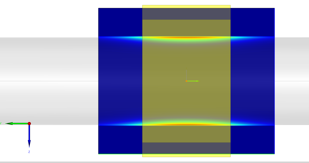
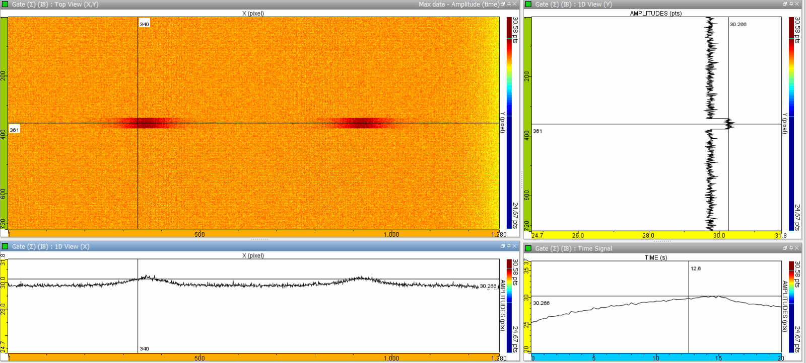
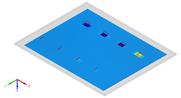
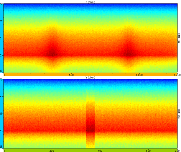
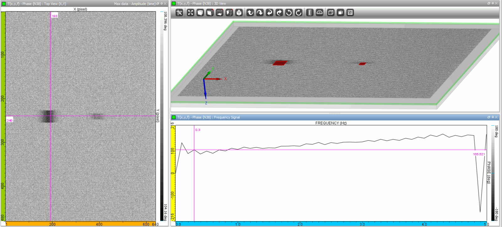
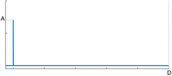
The thermogram at the component surface is displayed and can be superimposed to the 3D view. Thermograms are available in time domain or frequency domain (phase and amplitude). Temperature cross-section profiles along X or Y axis, and 2D maps along one axis and versus time are available.
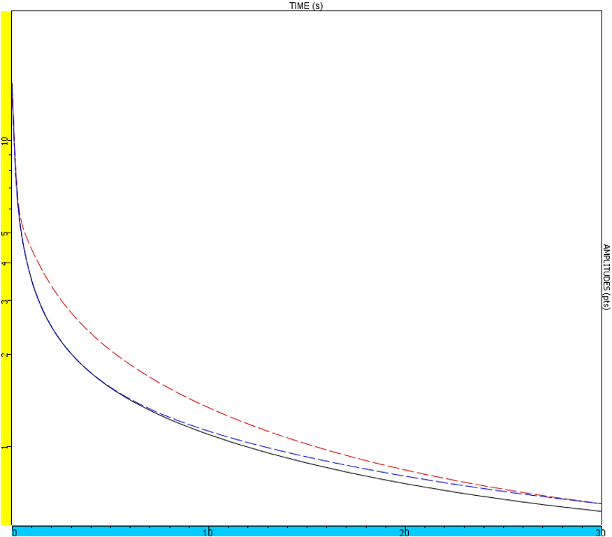
Time signal curves at any location in the component surface can be displayed in lin/lin, lin/log, log/lin or log/log scale. It can be also analysed in the Frequency Domain thanks to a FFT analysis.
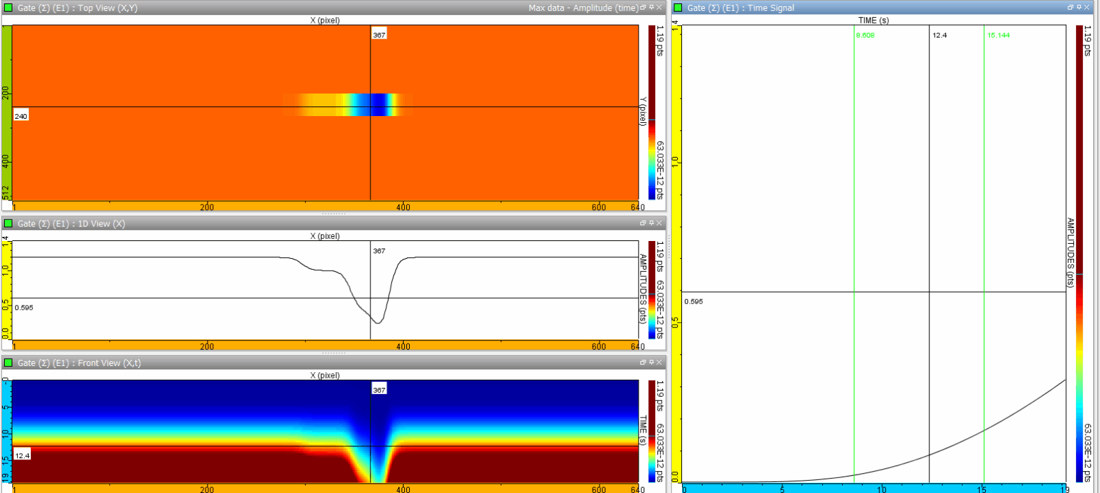
CIVA TT Simulation results: Thermogram (top left), Time signal curve (right), Cross section profile and map versus time (bottom left)
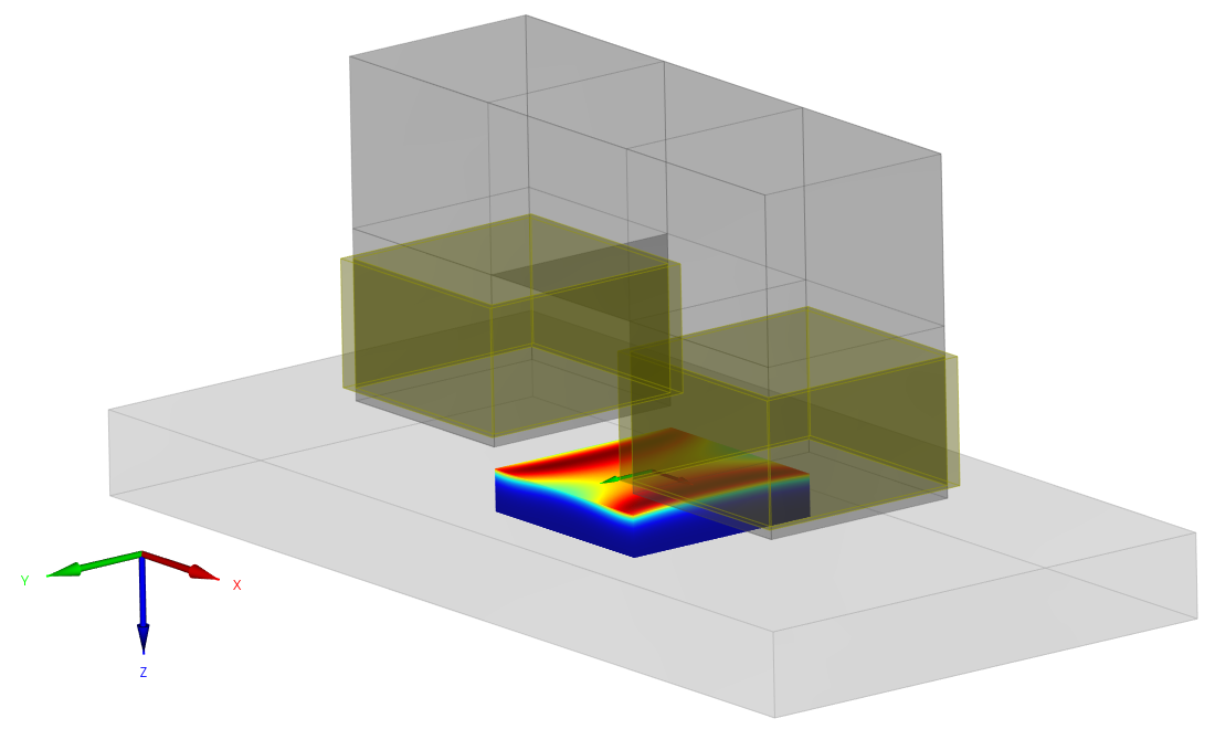
Induction Heating Computation
The Induction Heating module computes and displays the power density induced by an inductor supplied with a sinusoidal current at a given frequency. Depending on the type of inductors and specimen, semi-analytical or numerical techniques are used to solve Maxwell equations. The results are displayed in the 3D view or in the 3 crossed-planes of the computation area.