Inclusion in water - phased-array - Configuration without delay law

A reference for the relative amplitudes calculation has been choosen for each active aperture. It has been obtained comparing measure ans simulation results of the Ø2 mm SDH echoe at 8 or 12 mm depth, obtained varring the waterpath. The low SDH depth has been chosen in order to free us from the steel attenuation in simulations. Depending on the active aperture, the closest SDH which echo is not perturbed by the interface echo has been chosen:

• 20 elements aperture: SDH at 12 mm depth, 151 mm water path
• 16 elements aperture: SDH at 12 mm depth, 151 mm water path
• 12 elements aperture: SDH at 12 mm depth, 151 mm water path
• 8 elements aperture: SDH at 12 mm depth, 101 mm water path
• 4 elements aperture: SDH at 8 mm depth, 51 mm water path
• 1 elements aperture: SDH at 8 mm depth, 26 mm water path

The reference has been chosen at a waterpath for which SOV and SOV_COMPLETE models give the same results. The comparison of the amplitude/distance curves obtained for each aperture is presented from Figure 13 to Figure 15. The superimposition of measures and signals simulated with SOV_COMPLETE model at the reference is as well shown.

Note: the minimal acquired distance correspond to 1 mm water path relatively to the block surface. The echodynamic curves abscissa corresponds also to 1 mm wtaer path. 

The both SOV and SOV_COMPLETE models prédictions are globaly in agreement:: the SDH echo amplitude evolution is well reproduced. The amplitudes differences are very low for 1 to 8 mm elements apertures and appearing in the far field (around 2 dB overestimation).

For the apertures from 12 to 20 active elements, the same gaps disappear in far field. There may be an error on the attenuation value on water.  Note that the SOV_COMPLT new model improve the agreement between simulation and experiment at some water paths for 16 and 20 elements apertures (gaps reduced to 2 dB). 

In the case of the greatest aperture, différences appear at very low water paths and are not reduced with the SOV_COMPLETE model (gaps between 3 to 4 dB). For this case simulations have been carried out with greater accuracy (10), but the gaps is not reduced. 

The reference A-scans superimposition shows a good signal shape prediction.

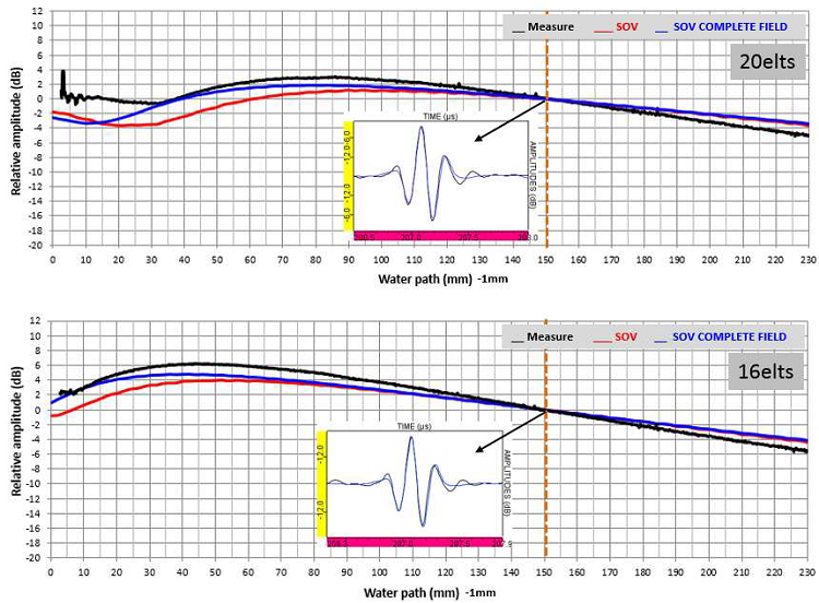
Figure 13 : Comparison of  measured and with SOV and SOV_COMPLETE simulated curves, Ø2 mm SDH at 8 mm depth. Phased array probes, 5 MHz, 20 and 16 elements aperture.

 

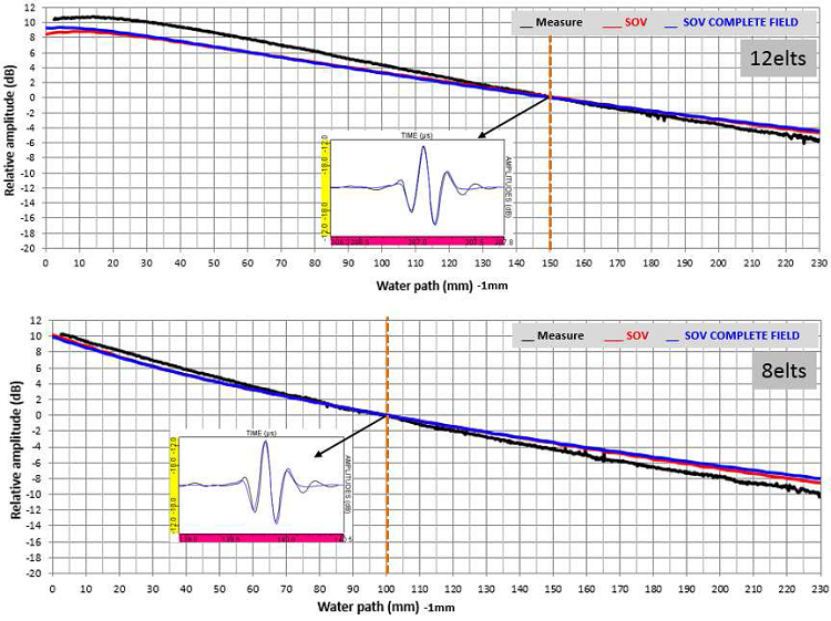
Figure 14 : Comparison of  measured and with SOV and SOV_COMPLETE simulated curves, Ø2 mm SDH at 12 mm depth. Phased array probes, 5 MHz, 12 and 8 elements aperture.

 

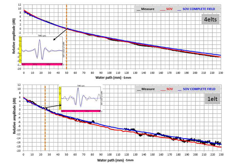
Figure 15 : Comparison of  measured and with SOV and SOV_COMPLETE simulated curves, Ø2 mm SDH at 12 mm depth. Phased array probes, 5 MHz, 14 and 1 element aperture.

Note : the experimental amplitude/distance curve presents some "holes" (lack of experimental data). Those data have been suppressed because they corrispond to areas where there is a mix between the specular echo on the SDH and a parasite echo (comming from another reflector, phantom echo ...). 

 

Figure 16 to Figure 18 show calculation result of field simulated in water with CIVA for all evaluated apertures. Under each field cartography (same dimensions for each apertures: 20 x 230 mm) is represented the ampliude/distance curve extracted at the aperture center. AT the right side of the cartography, it can be seen the profile in the plane perpendicular to the distance associated to the maximum amplitude.

The probe-inclusion distance for which the maximal amplitude of the emitted field is obtained, as well as the beam width at -3 dB are shown in the Table 1. As two amplitude maxima appear, both positions are measured.

For the biggest apertures (from 20 to 12 actibe elements), only one field amplitude maximum appears. For the lower amplitudes (from 8 to 1 elements), a second amplitude maximum appears, still located at the same water path. This second amplitude maximum, appearing for very different apertures in both directions (8 active elements: 4.7 x 10 mm²), is bounded by the probe dimension in the perpendicular plane (elements elevation: 10 mm).

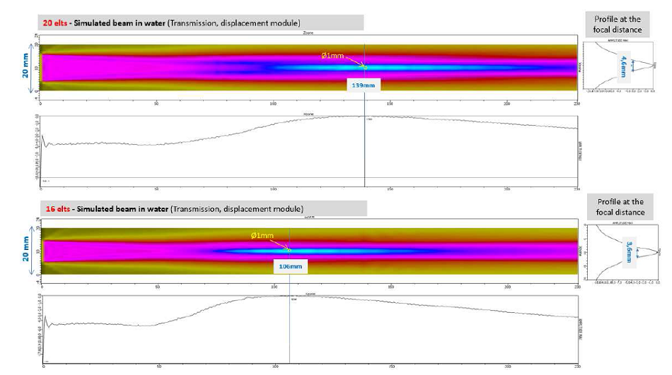
Figure 16: CIVA simulation of the field emitted by 20 and 16 active elements of the phased array probe in water. Phased array probe, 5 MHz. 

 

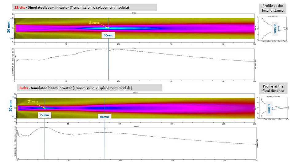
Figure 17: CIVA simulation of the field emitted by 12 and 8 active elements of the phased array probe in water. Phased array probe, 5 MHz. 

 

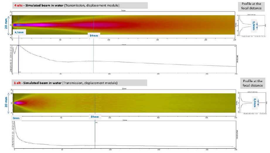
Figure 18: CIVA simulation of the field emitted by 14 and 1 active elements of the phased array probe in water. Phased array probe, 5 MHz. 

 

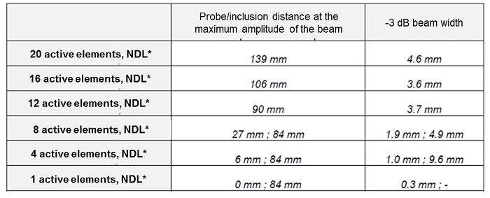
Table 1: Probe/inclusion distances corresponding to the field amplitude maximum emitted in the water on the probe axis and focal spot width as a function of the active aperture. Phased array probe with 20, 16, 8, 4 and 1 acive elements, without delay law.

 

*NDL = Null Delay Law

 

 

 amplitude/distance curves

The comparisons of the amplitude/distance curves measured and simulated with the three models SOV, SOV_COMPLETE and SPECULAR are presented Figure 19 (apertures of 20 to 12 elements) and Figure 20 (apertures of 8 to 1 elements).

 

Apertures of 20 to 12 elements 

A very good global agreement between the experiment and the simulation with the SOV_COMPLETE and SPECULAR models for the three apertures. The gaps don't exceed 2 dB. The agreement between the measure and the SOV model is not as well as both other models when the inclusion comes closer to the probe and that the probe aperture is great. The maximum gaps reach around 4 dB for the 20 elements aperture.

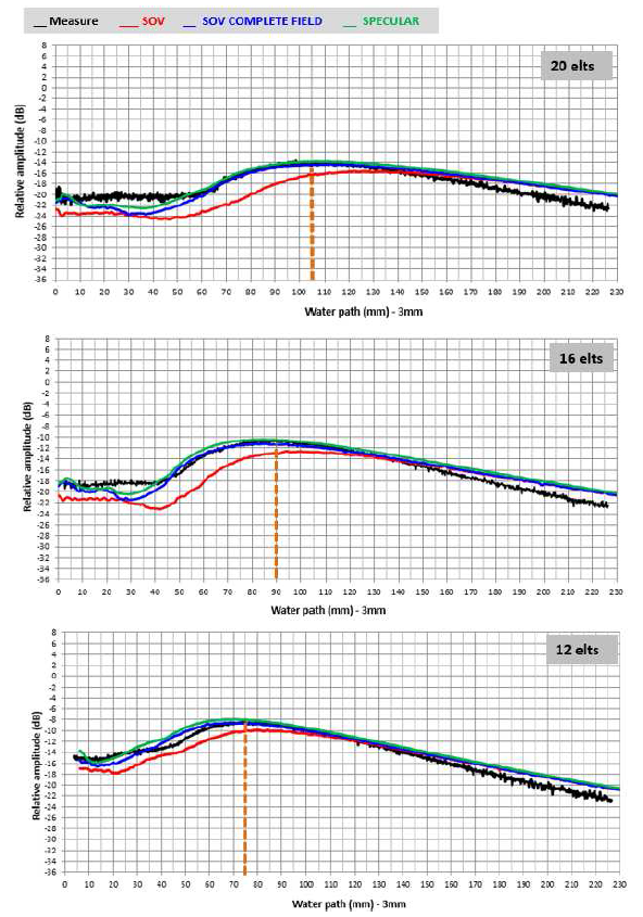
Figure 19: Comparisons of amplitude/distance curves measured and simulated in water with SOV, SOV_COMPLETE and SPECULAR models on a Ø1 mm inclusion, cases of 20, 16 and 12 elements apertures, without delay laws. Phased array probe, 5 MHz.

As we have noted on the amplitude/distance curves on SDH, the CIVA simulated amplitudes generally show a tendency to systematically overestimmate the amplitudes in far field (+2 dB to +3 dB). Those discrepancies can be attributed to an attenuation value error.

The « dmax » distance at which the echo amplitude is maximal is very well predited with SOV_COMPLETE and SPECULAR models for the 16 and 20 elements aperture. Differences don't exceed 1 mm. The position of the maximum is as well predicted for the 12 elements aperture, even if the gaps reach 5 mm. The SOV model has however a tendancy to overstimmate dmax of more than 10 mm with differences up to 20 mm for the greatest active aperture.

 

Apertures of 8 to 1 elements

We note as well a good prediction of the amplitude evolution as a function of the probe-inclusion distance with a systematic prediction of both amplitude peaks. However, the dmax distance position gaps are significant. CIVA underestimmates the distance. The gaps reach 13 mm for the 4 elements aperture with the SPECULAR model.

 

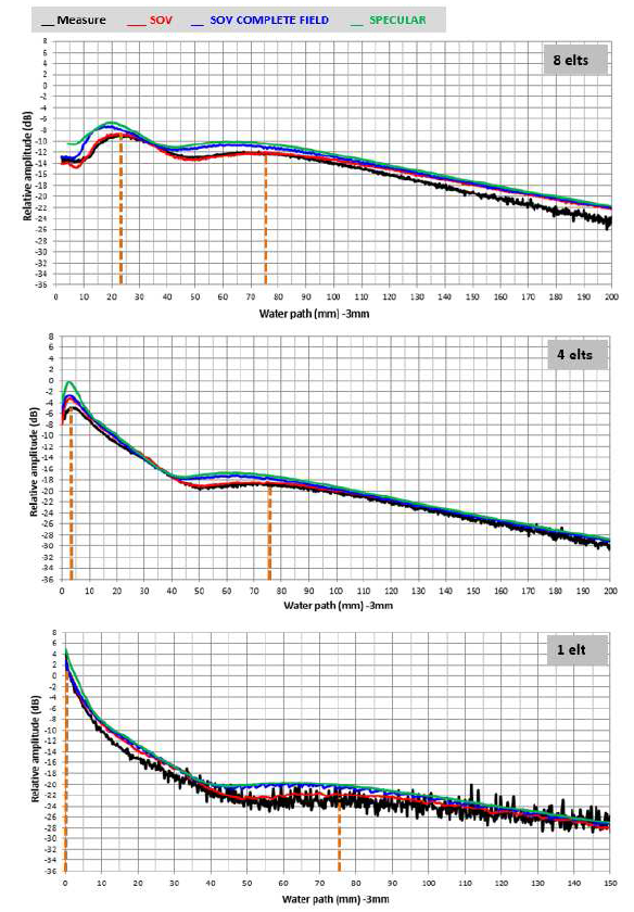
Figure 20 : Comparisons of amplitude/distance curves measured and simulated in water with SOV, SOV-COMPLET and SPECULAR models on a Ø1 mm inclusion, cases of 8, 4 and 1 elements apertures, without delay laws. Phased array probe, 5 MHz.

However, unlike the largest apertures (from 12 to 20 active element), the SOV model is the closest from the experiment with all lower apertures to predict the dmax distance and the amplitudes.

The low gaps obtained with SOV model compared to SOV_COMPLETE and SPECULAR models are surprising.SOV model lies on approximations stronger than SOV-COMPLET and is also supposed to be less accurate. In order to undestant those results, tests are presented here for the case of the 1 element aperture: the probe has been divided in several under-elements in order to carry out a computation channel by channel, limiting the approximations effects of the plane wave approximation of SOV model. The obtained results get closer to the ones obtained with SOV_COMPLETE and SPECULAR models. The good agreement between the three approaches suggests that the gaps are due to a common hypothesis to all CIVA models. The "piston"  hypothesis with a homogeneous displacement  on the surface of the sensor would be a possibility. It is indeed likely that the assumption that the sensor surface is similar to a set of uniformly distributed sources vibrating in phase and with the same amplitude, is not valid in particular when the surface of the element is small. The plane wave approximation of the SOV model would offset the effects of this hypothesis and would explain the best results obtained with low openings. However, it must be remembered that the gap remains acceptable with SOV_COMPLETE and SPECULAR models in the case of  reduced apertures without applying delay laws

The discrepancies between EXPERIMENTAL dmax and CIVA dmax are indicated in the Tabel 2. When two amplitudes peaks appear, both positions are given.

 

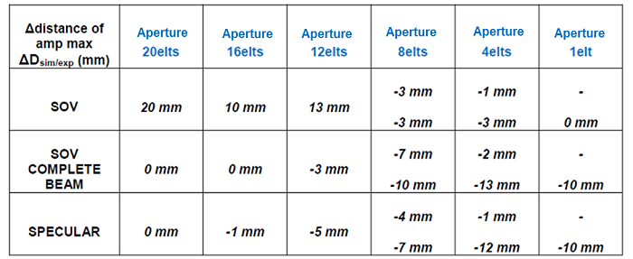
Table 2 : Differences (in mm) between simulations and measures for the probe/inclusion distances corresponding to the maximal amplitude emitted on the probe axis with SOV, SOV_COMPLET and SPECULAR models. Phased array probe, null dellay law, 5 MHz. 

 

Cartographies in the XY plane

The echodynamic curves in the XY plane has been extracted at the distances for which the amplitude of the amplitude/distance experimental curve is maximal. For those apertures for which two amplitude maxima are observed (apertures of 8, 4 and 1 elements), the extractions habe been realised at the two corresponding water paths. Moreover, as the probe dimensions are differents in both directions, the echodynamic curves along the probe incident plane (X axis) and the  plane perpendiculary to tje probe (Y axis) are presented.

The superimpositions of the experimental and SOV, SOV_COMPLETE and SPECULAR simulated curves are shown on the Figure 21 (apertures from 20 to 16 elements) and from the Figure 22 to the Figure 24 (apertures from 8 to 1 elements). Those curves are normalized in amplitude (max amplitude = 0 dB) in order to compare the focal widths.

 

Apertures of 20 to 12 elements:

The comparisons between experimental and simulated echodybamic curves normalized in amplitude following X and Y show a good agreement for the three models. The focal widths at -6 dB are correctly predicted with differences of +/- 0.5 mm.

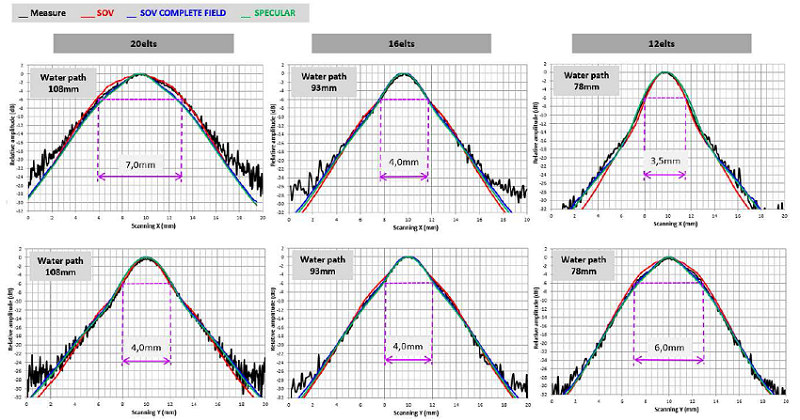
Figure 21 : Comparisons of amplitude/distance curves measured and simulated in water with SOV, SOV_COMPLETE and SPECULAR models on a Ø1 mm inclusion, cases of 20, 16 and 12 elements apertures, without delay laws. Phased array probe, 5 MHz.

 

Aperture of 8 elements:

 

• Along X axis: In the case of the probe-inclusion distance of 27 mm, a good agreement has been observed between the experimental echodynamic curves and with the 3 models simulated curves. At the second amplitude peak (probe-inclusion distance of 78 mm), the SPECULAR and SOV_COMPLETE models show the contribution of a « ray » type approach. Indeed, the SOV model tends to underestimmate the echoes amplitude as soon as the scanning along X axis get away from the probe center. 

• Along Y axis: The comparisons show that the 3 models predict echodynamic shapes similar and close to the experiment except for the SOV model at the water path of 78 mm where, unlike the extraction following X axis, the model tends to slightly overestimmate the amplitude, as soon as the scanning along Y move away from the probe center. 

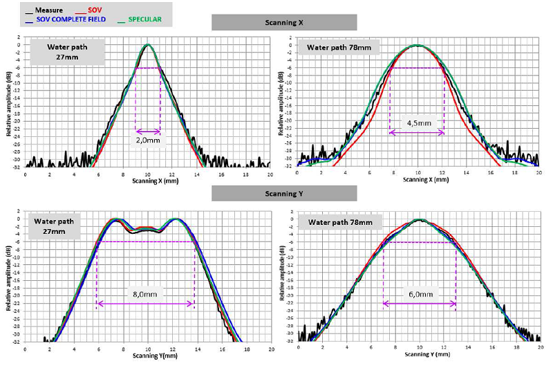
Figure 22 : Comparisons of amplitude/distance curves measured and simulated in water with SOV, SOV_COMPLETE and SPECULAR models on a Ø1 mm inclusion, case of 8 elements apertures, along X and Y axes. Phased array probe, 5 MHz.

 

Apertures of 4 and 1 element:

 

• Along X axis: In the probe incidence plane and for two water paths for which a maximal amplitude is observed, predictions of the focal width at -6 dB diverge from the experiment. The three models overestimmate the amplitude as soon as the position of the scanning moves away from the probe center. The focal width are overevaluated until +7.5 mm for SPECULAR model. This discrepancy is however predictable and can be associated to the approximation made on the piston probe vibration mode (particular velocity supposed uniformed on the piezo-electric surface). This approximation is not  valid when the aperture is very small. As in he case of the amplitude-distance curves, a lower disagreement with SOV model relatively to both other models is observed (SOV: +0.5 mm for a 3 mm inclusion-probe distance and +4.5 mm for 33 mm distance ; SOV_COMPLETE: +1.0 mm for a 3 mm inclusion-probe distance and +7.0 mm for 33 mm distance). As previously, tests habe been carried out and their results are in agreement with the idea that the SOV plane wave approximation offsets for this probe an error bounded to the hypothesis common to all others CIVA models.

 

• Along Y axis: For the three evaluated models, the echodynamic shapes are well predicted at both water paths (no gaps observed at focal width of -6 dB).

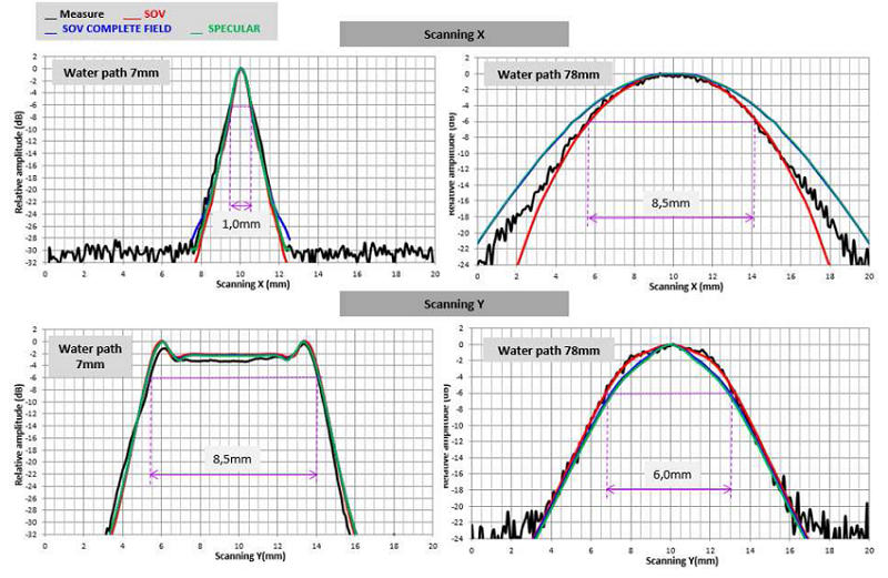
Figure 23 : Comparisons of amplitude/distance curves measured and simulated in water with SOV, SOV_COMPLETE and SPECULAR models on a Ø1 mm inclusion, case of 4 elements apertures, along X and Y axes. Phased array probe, 5 MHz.

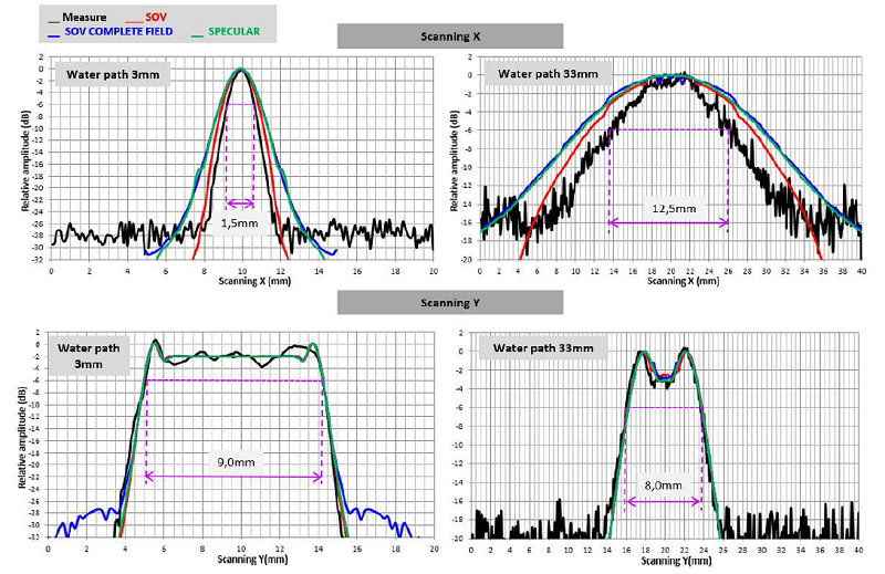
Figure 24 : Comparisons of amplitude/distance curves measured and simulated in water with SOV, SOV_COMPLETE and SPECULAR models on a Ø1 mm inclusion, case of 1 elements apertures, along X and Y axes. Phased array probe, 5 MHz.

 

The differences between the simulation and the experiment on focal width are shown on the Table 3 for the echodynamic curves following the probe incidence plane, the Table 4 for the echodynamic curves following the probe perpendicular plane.

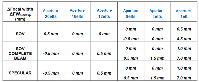
Table 3 : Differences (in mm) between the simulations and measures for the focal width at -6 dB along X at distances for which the maplitude/distance curve amplitude is maximal. Results of simulations with the three models. Phased array probe, null delay law, 5 MHz.

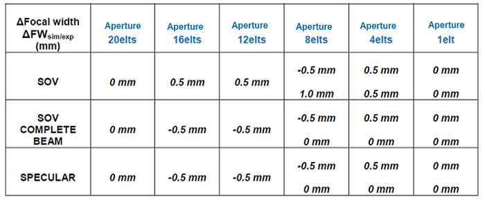
Table 4 : Differences (in mm) between the simulations and measures for the focal width at -6 dB along Y at distances for which the maplitude/distance curve amplitude is maximal. Results of simulations with the three models. Phased array probe, null delay law, 5 MHz.

 

The comparison of the experimental and  simulatedamplitude/distance curves in the infinite plane is presented Figure 25.

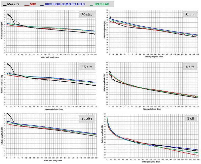
Figure 25 :  Comparison of amplitude/distance curves measured and simulated with SPECULAR,KIRCHHOFF and KIRCHHOFF_COMPLETE , infinite plane. Phased array probe, null delay law, 5MHz.

 

Note : unlike the acquisitions realised on the ball, the nearest acquiered water path is at 1 mm from the infinite plane. The absicissa indicated on the curves correspond also to the water path of less than 1 mm.

The comparisons of the experimental and simulated curves generally show a good prediction of the amplitude evolution as a function of the water path. In far field, we observe, as in the previous comparisons, an overestimation of around 2/3 dB that can be associated to an error on the attenuation value parameted in CIVA.

On the other hand, at low water path, we experimentally observe an important heightening of the surface echo amplitude, that is not reproduced by simulation. Experimental testings realised with a second probe, with equivalent characteristics (in gray dotted lines on the curves 20 and 16 elements), show that this heightening is different and also probably due to uncontrolled probe parameters.

In the case of only one active element, we observe in far field a stronger decreasing with KIRCHHOFF model relatively to both other models. The underestimation is around 4 dB for a water path of 230 mm. The decreasing of the echo amplitude of the infinite plane as a function of the water path is also slightly stronger with SPECULAR model, even if the underestimation at 230 mm is close to the experimental uncertainty. For KIRCHHOFF_COMPLETE model, the echo amplitude decreasing is quite well predicted. The maximal gaps are lower than 2 dB.

 

 

Effect of  an attenuation variation in water 

The whole obtained results shows systematic discrepancies between experiment and simulation in far field. The simulation tends to overestimmate the amplitudes. This tendency can be associated to an error on the attenuation value in water entered in CIVA. Computations have also been launched with another attenuation value. For the evaluation, we have selected the case of an aperture of 20 active elements. The attenuation value has also been adjusted in order that the amplitude measured on the reference (SDH located at 12 mm in the reference block) and the one obtained by simulation are in good agreement in far field. The obtained value is 0.02 dB/mm (the initial value was 0.005 dB/mm). The amplitude/distance curve also obtained on the reference is presented Fugure 26.

Only the results obtained with SOV_COMPLETE are presented.

Figure 26 :  Superimposition of amplitude/distance curves measured and with SOV_COMPLET simulated with attenuations of 0.005 dB/mm (literature) and of 0.02 dB/mm, SDH Ø2 mm at 12 mm depth in the feritic steel calibration block. Phased array probe 5 MHz, aperture of 20 elements. 

 

This on the reference adjusted value has then been reported in the simulation model of the 1 mm ball. The obtained amplitude/distance curve is presented Figure 27.

The results show a better agreement between the simulation and the experiment in far field. The agreement is also better at low water paths. The maximal observed gaps are lower than 2 dB.

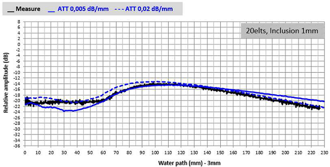
Figure 27 : Superimposition of amplitude/distance curves measured and with SOV_COMPLETE simulated in water on a Ø1 mm inclusion, attenuations of 0.005 dB/mm (literature) and of 0.02 dB/mm. Phased array probe 5 MHz, aperture of 20 elements. 

 

Study of the effect of a low central frequency variation 

As its influence is not negligible, we have evaluated the effect of a variation of 0.25 MHz (5% of the central frequency « fc » of 5 MHz used for the previous simulations) on simulation results.

The amplitude/distance curves calculated with the SOV_COMPLETE model for the three frequencies are represented Figure 28 (evolution on the calibration SDH at 12 mm depth) and Figure 29 (evolution of the amplitude on the inclusion). The reference for the aplitudes of each amplitude/distance curve obtained at a given frequency is the one of the SDH echo obtained at the same frequency.

The central frequency variation leads to an inclusions amplitude variation around the maximal amplitude (max +/- 1 dB) and the probe/inclusion distance corresponding to the maximal amplitude (around 2 mm). Those variations can be considered as uncertainties on CIVA simulation results related to the uncertainty on the central frequency value of the entry signal.

 

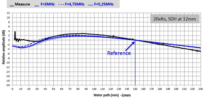
Figure 28: Superimposition of measured and with SOV_COMPLET simulated amplitude/distance curves for the Ø2 mm SDH at 12 mm depth in the ferritic steel calibration block. Those comparisons show that the values and positions of  amplitude/distance curves maxima depends on central frequencies of the entry signal of 4.75 and 5.25 MHz. Phased arry probe, 5 MHz, aperture of 20 elements.

 

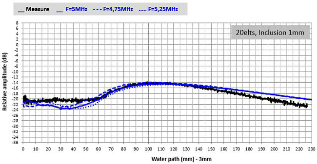
Figure 29: Superimposition of measured and with SOV_COMPLETE simulated amplitude/distance curves for the Ø1 mm inclusion. Those comparisons show that the values and positions of  amplitude/distance curves maxima depends on central frequencies of the entry signal of 4.75 and 5.25 MHz. Phased arry probe, 5 MHz, aperture of 20 elements.