Inclusion in water - phased-array - Simulation settings

Several "development" versions of CIVA were used for the simulations due to corrections or optimizations on new models evaluated for phased array. The last version used is the development version of November 6, 2015.

SPHERICAL STEEL INCLUSIONS

The models used for calculating the echoes of the spherical steel inclusion placed in water are:

• SOV (Separation Of Variables)
• SOV_COMPLETE (Separation Of Variables without plane wave approximation for the incident field on the defect). This new model is not present in the current commercial version of CIVA that is why we used the development version.
• SPECULAR

These various models are discribed HERE.

The assumptions and approximations related to each model result in a different range of validity for each of them. Thus, in CIVA, depending on the ratio between the center frequency of the probe and the size of the spherical inclusion, the three models listed above may (or not) be allowed. The bridles CIVA 2015a are:

• for SOV : bridle for k*radius>20 where k is the wave number. The condition is realised for vL and/or for vT accoding to the requested modes.
• for SPECULAR : warning for k*radius<20, but the calculation may be run.
• for SOV_COMPLETE: same warnings as for SOV but no bridle, the calculation is possible. 

In the case of  configurations of validation with the phased-array probe, 5MHz, only a warning appears with the SPECULAR model.

For achievable CIVA 2015a simulations (SOV and SPECULAR echoes), we verified that the results of CIVA 2015a are identical to those of the development version.

 

INFINITE PLANE

The models used to calculate the echoes of the infinite plane are SPECULAR model,  KIRCHHOFF and KIRCHHOFF_COMPLETE. 

 

Side drilled holes (SDH)

These reflectors placed at different depths in the ferritic steel calibration specimen were used to calibrate the probes.

To simulate the SDH echoes, the SOV and SOV_COMPLETE models were used. In CIVA 2015a, the bridles for these reflectors are:

• For SOV: no bridle for large SDHs even if this model is less accurate for them.
• For SOV_COMPLETE: same as SOV

Note : The accuracy for beam and defect response used for the simualtions were sometimes set to 10 and 10 in order to ensure convergence of the results.

 

 

DETERMINATION OF SIGNAL PARAMETERS INPUT IN CIVA

Unlike previous validation studies, the adjustment of the center frequency is not performed because it depends on the reference reflector used (FBH or SDH or surface echo ...) and the selected model to calculate the reference echo (SOV, SOV_COMPLETE, KIRCHHOFF, KIRCHHOFF_COMPLETE, SPECULAR ...). This dependence is due to the fact that the echoes predicted for different reflectors by the different models of CIVA are based on different approximations due to the assumptions of each model. Thus, it is not possible to define a central frequency obtained by adjusting and that would be common to all models. In addition, the method also depends on the reliability of the acquisition of the reference echo. Therefore, the central frequency of the input signal in CIVA corresponds to the nominal frequency (5 MHz).

The other two signal parameters, the bandwidth and phase are always determined by adjusting the temporal shapes of the measured and simulated echoes from a reference reflector for which CIVA predictions have been validated. The reference reflector chosen for this probe is a SDH of 2mm diameter located in a homogeneous ferritic steel calibration block. This reference echo has been measured for a water path of 150mm.

The bandwidth and phase of the input signal determined are:

• Bandwidth = 65%
• Phase = 330°

Figure 10 shows an example of superimposition of experimental and simulated (with SOV_COMPLETE model) echoes of a  Ø2mm SDH loacted at 12mm depth.

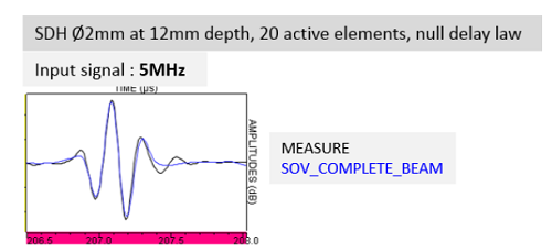
Figure 10 : Adjustment of the CIVA input signal so that the experimental and simulated with SOV_COMPLETE  A-scans of a Ø2mm SDH loacted at 12mm depth in a steel calibration block so they are are in good agreement. Normalized amplitudes. Phased-array probe, 5MHz, 20 active elements, null delay laws, L0 °, water path 150mm

 

 

PARAMETERS OF WATER

The velocity in the water was measured experimentally using successive skips of a surface echo on an infinite plane.

• vLwater = 1483 m/s

The attenuation in the water has been taken into account. The value of the attenuation coefficient of the L wave in water at a frequency of 5 MHz set in CIVA is:

• coeffAttenuation = 0.005 dB/mm

This value from literature was validated during the validation of  inclusions responses detected with a single-element probe in immersion (here). The experimental and simulated results of the echo of a Ø2mm SDH were compared while varying the water path.

 

Delay laws

The delay laws used in simulation are the same as those calculated and applied in the acquisition system. The settings have been set by defining in the model a specimen made of water, the probe was positioned at a short distance from the mock-up. The focal point is at 30mm depth in the component made of water and with the probe positioned 3mm from the part. The focal depth is then 33mm. An example of the delay laws calculated for a configuration with 32 active elements and a focus at 33mm is presented Figure 11.

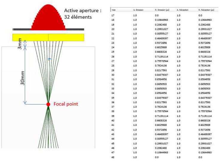
Figure 11 : Delay laws calculated for focusing at 33mm in water L0 °. Phased-array probe, 5MHz, configuration with 32 active elements.

 

In CIVA, in order to simulate mapping of inclusions, you must define a specimen which material is fluid type (water) and in which you will place the steel inclusions.

Moreover, XZ mappings are particular : CIVA can simulate them using a CAD part of plane geometry (which material is fluid) and choosing the probe positioning by the cristal center. The displacement is shown in Figure 12. This type of mapping can not be simulated using a flat piece.

 

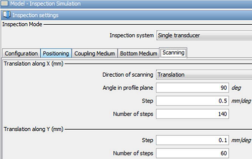
Figure 12 : Configuration of the scanning for simulation of the  XZ or YZ mappings with CIVA.