Entry parameters in CIVA
- Probe diameter: 9.5 mm
The central frequency of the entry signal is the nominal probe frequency:
- Central frequency = 10 MHz
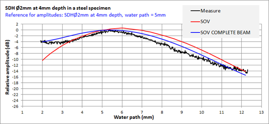
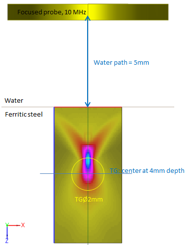
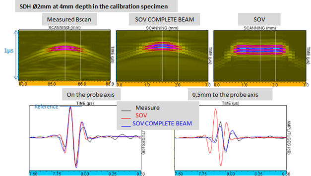
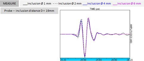
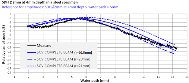
The Bandwidth and the phase of the entry signal are determined by adjustement of the temporal shapes of a measured and SOV_COMPLET simulated echoes (Figure 56) of a side drilled hole located at 4 mm depth in the calibration steel block and obtained for a 5 mm water path.
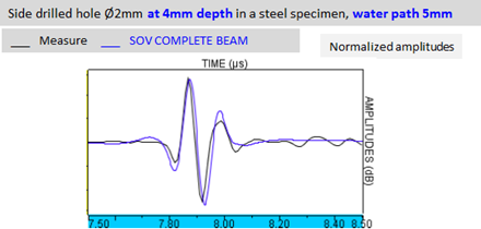
The entry signal bandwidth and phase also determined are:
- Bandwidth = 65%
- Phase = 300°
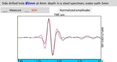
Those values lead to a good agreement between experimental and SOV_COMPLET (Figure 56) and SOV (Figure 57) simulated A-scans even if the SOV_COMPLET echo is a little too much "low frequency".
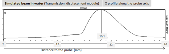
The curvature radius has been determined by adjustment of the focal distance predicted by the CIVA beam computation with the one indicated by the manufacturer (0.8 inch also 20.3 mm). The probe field in water after this adjustment is presented Figure 58.
- Curvature radius = 20.5 mm
The attenuation in water has been taken into account, the L waves attenuation coefficient value in water at 10 MHz frequency defined in CIVA comes from the Literature.
- coeffAttenuation = 0.022 dB/mm
AMPLITUDES references for MEaSURE/CIVA comparisons
reference choice
The reference choice for these amplitudes has been problematic for this probe because:
- Unlike previous probes, usual reference reflectors echoes (SDH or FBH) simulated with focused probes have not been experimentally validated yet.
- The SOV and SOV_COMPLET simulated SDH echoes are not identical even for tne FBH located at the field focal distance in the piece.
- The amplitude ratio between SDH and FBH echoes of calibration blocks obtained with CIVA are not in agreement with the measure. Consequently, depending on the choice of the reference reflector, SDH or FBH, a gap between experimental and simulated inclusions amplitudes is observed.
For those reasons it has been decided:
- to choose a SDH as reference rather than a SDH to be homogeneous with previous probes references and to evaluate with complementary measures the SOV and SOV_COMPLET simulated SDH echoes validity.
- to choose as reference for amplitudes for inclusions echoes obtained with a SOV (or SOV_COMPLET) model the reference SDH echo amplirtude obtained with this model SOV (or SOV_COMPLET). We remind that for both previous plane probes, SOV and SOV_COMPLET model predicted same amplitude as the reference echo and consequently these distinction was not necessary. For the inclusions echoes obtained with SPECULAR, the SDH echo amplitude obtained with SOV_COMPLET will be consider as reference (the SDH echoes can not be calculated with SPECULAR in CIVA).
- to indicate the discrepancies between the measured and simulated amplitude ratio SDH/FBH and to represent some comparison results of inclusions experimental and simulated amplitude/distance curves when a FHB is used as reference.
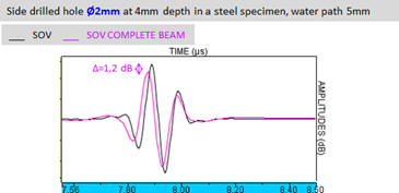
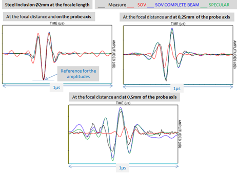
The reference is the L0° specular echo amplitude of the Ø2 mm SDH located at 4 mm in the calibration block inspected with a 5 mm water path. For this reference SDH, which has been used to determine entry signal phases and bandwidths, SOV and SOV_COMPLET models simulate echoes with a similar shape but no different amplitude (Figure 59). Consequently:
- the reference for the inclusions echoes amplitudes obtained with SOV is the reference SDH echo amplitude obtained with this model.
- the reference for the incusions echoes amplitude obtained with SOV_COMPLET and SPECULAR and infinlte plane echoes obtained with SPECULAR is the reference SDH echoes amplitude obtained with SOV_COMPLET.
experimental Validation of the SDh reference echo
For this validation, experimental and simulated amplitude/distance and XY curves of the reference SDH have been compared.
-
Amplitude/distance curve, reference reflector case
The SOV_COMPLET simulated amplitude/distance curve of the reference SDH is quite similar of the one measured while the SOV simulated curve differs by more than 2 dB from measure (Figure 60).
-
XY curve, reference reflector case
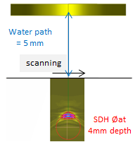
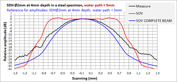
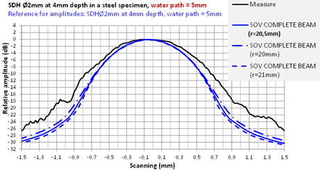
The XY curve has been acquiered for a 5 mm water path chosen in order that the SDH shining point is located at the focal distance in the calibration block (Figure 61). The configuration is represented Figure 62.
The SOV simulated XY curve is absolutly not in agreement with the measure when the SDH moves away from the probe axis (Figure 63, red curve). However, the SOV_COMPLET curve shape is much closer to the measure even if discrepancies are greater than 2 dB when the inclusion is shifted more than 0.5 mm from the probe axis (Figure 63, blue curve). B-scans and A-scans presented on the Figure 65 illustrate as well the most important gaps for SOV which are explained by the fact that the plane wave approximation considered by the model is not as much valid as the SDH moves away from the probe axis.
Although those differences between measurements and SOV and SOV_COMPLET simulations for the reference SDH, this SDH has been chosen as reference because of a lack of a "better" reference.
beam of the focused probe 10 MHZ in water
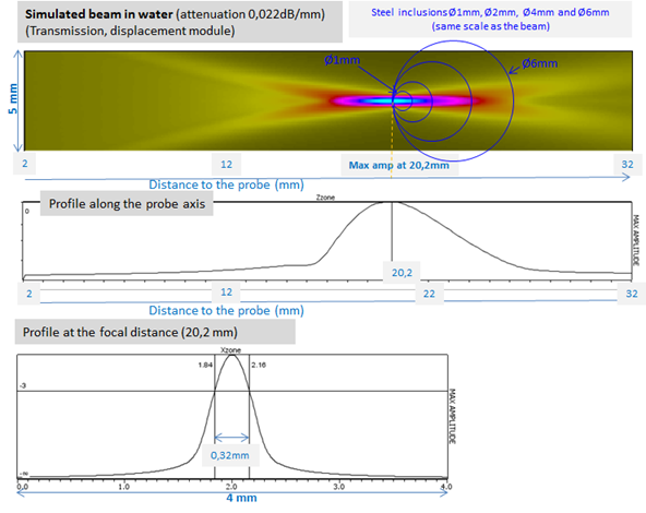
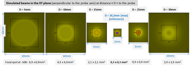
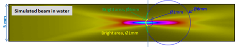
The maximal amplitude emitted by the probe on its axis is located at a 20.2 mm distance. The focal spot width at -3 dB, for this distance, is 0.3 mm.
All the balls are also much greater than the focal spot (Figure 65 on the top).
results obtained for steel inclusions
|
10MHZ |
Inclusion Ø 1mm |
Inclusion Ø 2mm |
Inclusion Ø 4mm |
Inclusion Ø 6mm |
|
SOV |
no |
no |
no |
no |
|
SOV_COMPLET |
no |
no |
no |
no |
|
SPECULAIRE |
yes |
yes |
yes |
yes |
experimental results
The experimental amplitude/distance echodynamic curves obtained for the 4 inclusions are presented on Figure 67. On the upper graph, the amplitudes are relative to the reference echo amplitudes (Side drilled holes SDH); at the bottom the amplitudes are normalized.
- The echoes maximal amplitude increases by around 6 dB when the inclusion diameter increases from 1 to 2 mm. The rise is equal to 2 dB when the diameter increases from 2 to 4 mm. The amplitude remains constant between the 2 and 4 mm inclusions.
- The « dmax » distance at which the echo amplitude is maximal depends on the inclusion (see further table).
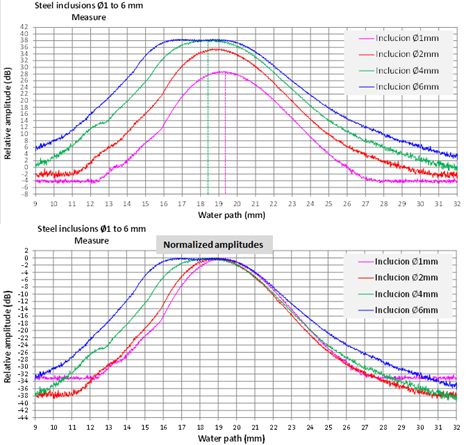
The XY experimental curves obtained for the 4 inclusions at the experimental focal distance are presented on the Figure 68 (normalized amplitudes).
- The focal spot width depends on the inclusion diameter.
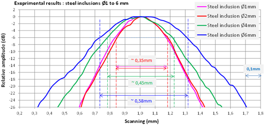
- However, the shape of the Ø1 to Ø6 mm inclusions specular echoes located at 19 mm do almost not depend on the inclusion diameter (Figure 69).
MEaSURE/CIVA Comparison
-
Amplitude/distance curve
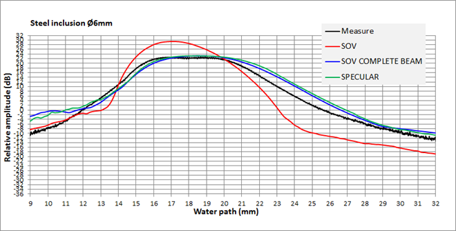
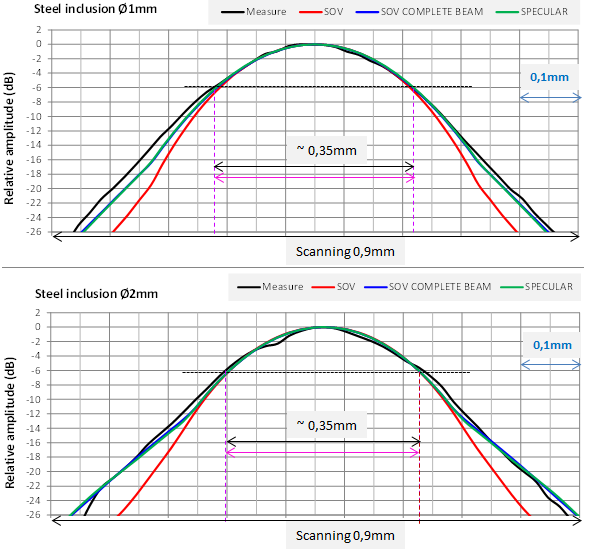
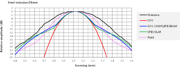
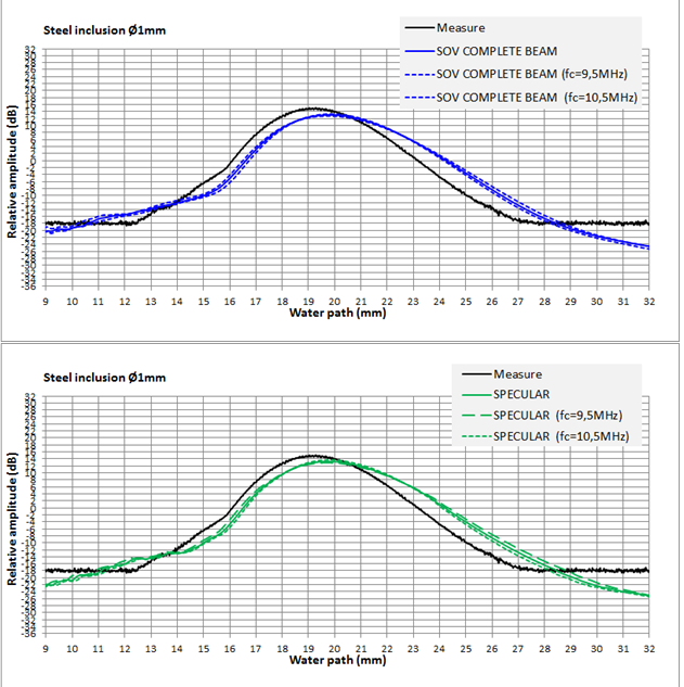
The comparisons of SOV, SOV-COMPLET and SPECULAR simulated and experimental amplitude/distance curves have been studied for all inclusions diameters. The Figure 70 shows the results obtained with the Ø1 mm inclusion. The Figure 71 shows the results obtained with the Ø6 mm inclusion.
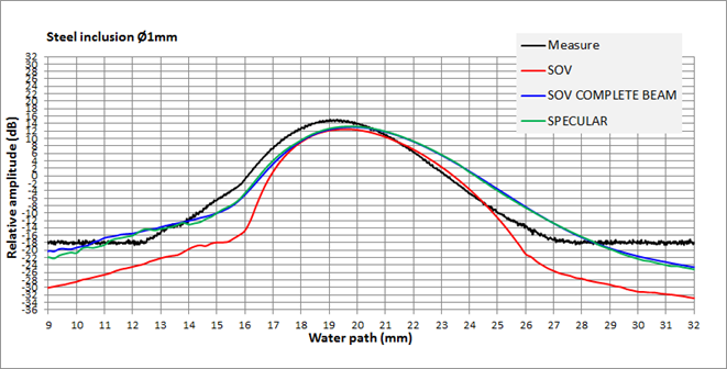
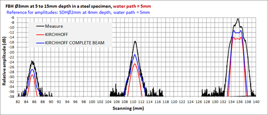
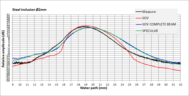 Figure 71: Comparisons of SOV, SOV-COMPLET and SPECULAR simulated and experimental amplitude/distance curves, Ø2 mm inclusion. Reference for the amplitudes: L0° echo of a Ø2 mm SDH at 4 mm depth in the calibration block, 5 mm water path. In the commercial CIVA version, only the SPECULAR model is allowed for the Ø2 mm inclusion. Ø9.5mm focused probe, 20.5 mm curvature radius, 10 MHz.
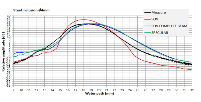 Figure 72: Comparisons of SOV, SOV-COMPLET and SPECULAR simulated and experimental amplitude/distance curves, Ø4 mm inclusion. Reference for the amplitudes: L0° echo of a Ø2 mm SDH at 4 mm depth in the calibration block, 5 mm water path. In the commercial CIVA version, only the SPECULAR model is allowed for the Ø1 mm inclusion. Ø9.5mm focused probe, 20.5 mm curvature radius, 10 MHz.
At the dmax distance, the maximal amplitude/distance curve amplitude is indicated in the Table 13.
The differences between dmaxEXPERIMENTAL and dmaxCIVA are indicated in Table 14.
|
Distance “D” of amp max (mm) |
Simulated beam |
Inclusion Ø1mm |
Inclusion Ø2mm |
Inclusion Ø4mm |
Inclusion Ø6mm |
|
|
20.2 |
|
|
|
|
|
Measure |
|
19.3 |
19.1 |
18.6 à 18.9 |
17 à 19.5 |
|
SOV |
|
19.4 |
19.2 |
18.2 |
17 |
|
SOV_COMPLETE_BEAM |
|
19.8 |
19.6 |
19 à 19.2 |
18 à 19.5 |
|
SPECULAR |
|
19.8 |
19.6 |
19 à 19.2 |
18 à 19.5 |
|
Δdistance of amp max ΔDsim/exp (mm) |
Inclusion Ø1mm |
Inclusion Ø2mm |
Inclusion Ø4mm |
Inclusion Ø6mm |
|
SOV |
- |
- |
- |
- |
|
SOV_COMPLETE_BEAM |
0.5 |
0.5 |
0.4 |
0.5 |
|
SPECULAR |
0.5 |
0.5 |
0.4 |
0.5 |
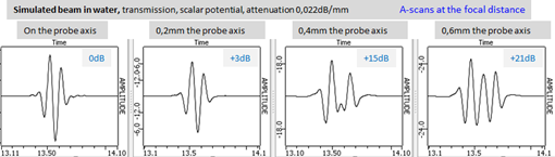
SOV model: the shapes of the experimental and SOV simulated amplitude/distance curves are very different. The difference increases when the incusion diameter increases. Indeed, the inclusion surface contributing to the echo increases as well as the inclusion part located off axis (Figure 74) for which the plane wave approximation doesn't allow a correct description of the incident field. A-scans of field emitted in water for 4 points located at the focal depth (a point on the probe axis and 3 others shifted from the axis by 0.2, 0.4 and 0.6 mm) have been represented (Figure 75) to illustrate the signal complex shape when the observation point deviates from the axis.
SOV_COMPLET and SPECULAR models: both models almost give same results. SOV_COMPLET and SPECULAR amplitude/distance curves shape are much closer to the experimental curves the SOV curves. However, around 0.5 mm differences between dmaxEXPERIMENTAL and dmaxSOV_COMPLET (or dmaxSPECULAR which is identical) (Table 13 and Table 14) and very important discrepancies for the greater distances dmax.. Those differences which can reach 8 dB are partly due to the dmax. shifting.
Those experiment/simulations comparisons point out the SOV_COMPLET contribution compared to SOV. They show as well that the current restrictions in CIVA are justified for SOV but not necessary for SOV_COMPLET which gives results close to SPECULAR. The restrictions for SOV_COMPLET exist to avoid numerical problems of coefficients calculations (suspected to be the cause of the observed gaps for the great inclusions). A more detailled analysis of this problem could allow to better define the restrictions of SOV_COMPLET which should be less strict than those of SOV.
-
Cartographies in the XY plane at the focal distance
For each inclusion, the experimental XY curves have been extracted at the distance for which the maximal amplitude had been observed in the XY plane (=dmaxEXPERIMENTAL). The simulated XY curves have been extracted at the same positions. Those curves are normalized in amplitude (max amplitude = 0 dB). The comparisons (Figure 76, Ø1 and Ø2mm inclusions) and Figure 77 (Ø4 and 6mm inclusions) show:
- Ø1 and 2mm inclusions:
- a good agreeemnt with the measurement for SOV_COMPLET and SPECULAR models on the whole scanning (around 0.8mm).
- a good agreeemnt with the measurement for SOV only when the inclusions are located within 0.2 mm from the probe axis, beyond SOV underestimates the amplitudes.
- the focal spots width simulates with the 3 CIVA models at -6dB are close to the measure: 0.35mm.
- Ø4 and 6mm inclusions:
- the 3 models don't correctly predict the inclusions echoes amplitudes when they deviate from the probe axis.
- In the SOV case this is mainly because the plane wave approximation is less valid when the SDH deviates from the probe axis.
- In the SOV_COMPLET and SPECULAR case, the XY curves shape shows an « unhooking » which is experimentally not observed and which seems to be the cause of discrepancies with measurements. The experiemental focal spots widths are 0.45 mm and 0.58 mm for the Ø4 and Ø6 mm inclusions, while following SOV_COMPLET and SPECULAIRE they are 0.33 and 0.34 mm.
- the 3 models don't correctly predict the inclusions echoes amplitudes when they deviate from the probe axis.
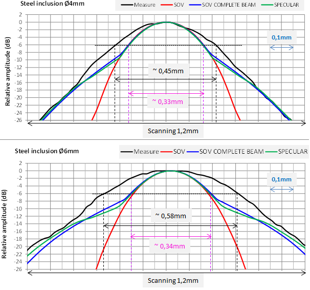
The low « unhooking » observed on the XY curves predicted by SOV_COMPLET and SPECULAR for the Ø4 and 6 mm inclusions is obtained when the inclusion center is shifted by 0.2 mm from the probe axis. It seems not to be caused by an amplitudes « unhooking » of the field emitted which decreasing on either side of the probe axis at the focal distance is very regular (Figure 78). Its origin has to be studied.
The experimental and with the 3 models simulated A-scans confirm that the SOV_COMPLET and SPECULAR predictions are more correct that the one simulated with SOV when the inclusion is not on the probe axis (Figure 79).
results obtained for the infinite plane
SPECTRum of the small inclusions echoes and of the infinite plane
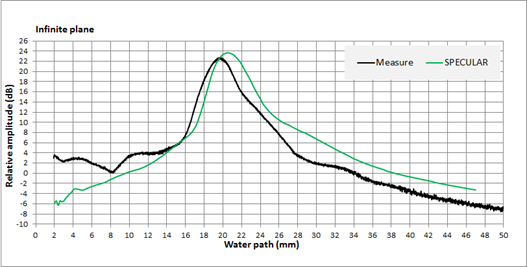
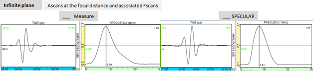
- measured and SPECULAR simulated spectra of the infinite plane at respectively dmaxEXPERIMENTAL and dmaxSPECULAR (Table 15).
- measured and SOV_COMPLET and SPECULAR simulated spectra of Ø1 mm and Ø4 mm inclusions, at respectively dmaxEXPERIMENTAL, dmaxSOV_COMPLET and dmaxSPECULAR (Table 16).
Infinite plane: the central frequency predicted by the SPECULAR model is closed to the measured one but different from the probe nominal frequency (around 8 MHz instead of 10 MHz). Measured and SPECULAR simulated are also quite similar. The whole experimental and SPECULAR simulated spectra (Figure 81) shows a different frequencies.
|
Infinite plane at the focale distance |
||
|
|
fc (MHz) |
BW (MHz) |
|
Measure |
8.4 |
6.5 |
|
SPECULAR |
7.9 |
6.3 |
As previously seen, the SOV_COMPLET and SPECULAR simulated inclusions echoes, located at dmaxSPECULAR (= dmaxSOV8COMPLET) are similar. The central frequency and bandwidth extracted from their spectra are also close the measured ones.(Table 16).
|
|
Steel inclusion Ø1mm at the focal distance |
Steel inclusion Ø4mm at the focal distance |
||
|
|
fc (MHz) |
BW (MHz) |
fc (MHz) |
BW (MHz) |
|
Measure |
8.9 |
6.8 |
8.6 |
6.2 |
|
SOV-COMPLETE-BEAM |
9 |
6.4 |
8.6 |
6.3 |
|
SPECULAR |
8.8 |
6.5 |
8.4 |
6.2 |
effect of a low VARIATION of the central frequency
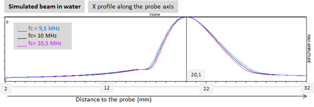
For both new frequencies (9.5 and 10.5MHz) the probe curvature radius to define in CIVA has to be determined following the method (described in the simulations descriptions chapter). It consists to adjust the curvature radius value in order that the focal distance in water according to a CIVA field calculation is the one indicated by the manufacturer. As the position of the maximal amplitude of the emitted field by the probe in water on its axis doesn't change when the probe central frequency is modified by 0.5 MHz (Figure 82), the curvature radius to define for the calculations at 9.5 MHz and 10.5 MHz are the same as the one determined at 10 MHz.
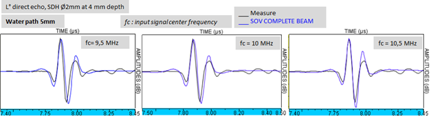
The experiment/simulation agreement for the reference echo (Ø2 mm SDH at a 4 mm depth insepcted with a 5 mm water path) for the 3 frequencies (9.5 MHz, 10 MHz and 10.5 MHz) is verified (Figure 83). The SDH echo obtained with the entry signal at 10 MHz was already too low frequency, the SOV_COMPLET/measure difference is also increased with the 9.5 MHz entry signal and reduced with the 10 MHz one. The SOV_COMPLET/measure agreement at the 3 frequencies is satisfying enough to calculate the amplitude/distance and XY curves.
The amplitude/distance curves calculated with SOV_COMPLET and SPECULAR models for the 3 frequencies are represented Figure 84 for the Ø1 mm inclusion. The reference for the amplitudes of each amplitude/distance curves obtained at a given frequency is the SDH echo amplitude obtained at the same frequency.
Those results show that the central frequency variation lead to low variations which doesn't change the observations and conclusions done so far with the 10 MHz entry signal.
effect of a low variation of the crystal curvature
Fort hose 2 new 20 mm and 21 mm curvature radii, focal distances in water are respectively equal to 19.6 mm and 20.6 mm. It was 20.2 mm for the 20.5 mm radius.
results obtained with 3 similar curvature radii
The experimental and SOV_COMPLET simulated amplitude/distance curves for the 3 curvature radii are plotted Figure 83 (Ø1 mm, 4 mm and 6 mm inclusions). The reference for the amplitudes of each curve is the SDH echo amplitude obtained with the same curvature radius.
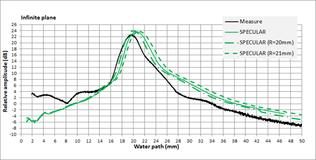
Those results show that the curvature radius variation has important effects on the curves. For the 3 inclusions, SOV_COMPLET predictions with the 20 mm curvature radius are the closest to the measure. For this curvature radius, dmaxEXPERIMENTAL and dmaxSOV_COMPLET are quite identical and the observed differences for the greater distances are around 2 to 4 dB (Ø4 mm inclusion beyond dmax). The amplitude/distance curve of the infinite plane calculated with the SPECULAR model and the 20 mm curvature radius is closer from the experimental results compared to the curve obtained with the 20.5 mm radius. However, it still remains a discrapancy between dmaxEXPERIMENTAL and dmaxSPECULAR (Figure 83).
Otherwise we have compared SDH reference echoes with SOV_COMPLET for 20 mm and 21 mm curvature radii (Figure 86 and Figure 87): the amplitude/distance curve (Figure 86) and the XY curve (Figure 87) are still close to the measure for the 20 mm curvautre radius. But the simulated XY curve with the 21 mm radius deviates from measurement.
FBH reference
The important discrepancies are not reduced when the simulations are realized with the 20 mm curvature radius for which the inclusions echoes simulation with SOV_COMPLET and of the infinita plane with SPECULAR were closer to the measure than the ones realized with a 20.5 mm radius.
If instead of the SDH we would ahve chosen the Ø3 mm FBH at 5 mm depth as amplitudes reference, discrapancies would have been much greater: a 6 dB offset (resp. 8 dB) would have been noted on SOV_COMPLET or SPECULAR (resp. SOV) simulated amplitude/distance curves. Consequently, characterization study of SDH and FBH responses of calibration blocks with focused probes is necessary.
Synthese
Continue towards Conclusion
Back to Results obtained with the 5 MHz probe
Back to Single element probe