
Inclusion in water – single element – 5 MHz probe
Summary
- Input parameters in CIVA
- Probe parameters
- reference for the amplitudes while MEaSURE/CIVA comparisons
- Beam of the 5 MHz probe in water
- results obtained for steel inclusions
- experimental results
- MEaSURE/CIVA comparisons
- Results obtained for the infinite plane
- echoes spectrum of the inclusions and the infinite plane
- EFFEcT of a poor variation in the central frequency
- Synthesys
Input parameters in CIVA
Probe parameters
The CIVA entry signal parameters for the 5 MHz probe have been determined in the same way as the 2.25 MHz probe.
The central frequency is the one given by the manufacturer:
- Central frequency = 5 MHz
The bandwidth and the phase are determined by adjustments of temporal shapes of measured and with COMPLETE_SOV simulated echoes of the Ø2 mm SDH located at 8 mm depth in the stell calibration block. The reference echo has been measured for a water path of 29 mm (Figure 35).
The entry signal bandwidth and phase also obtained are:
- Bandwidth =65%
- Phase = 290°
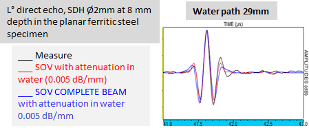
Figure 35 : Superimposition (after adjustments) of CIVA entry signal bandwidth and phase of measured and with SOV and COMPLETE_SOV simulated A-scans of a Ø2 mm SDH located at 8 mm depth in the stell calibration block, water path of 29 mm. Normalized amplitudes. Ø6.35 mm plane probe, 5 MHz.
The attenuation in water has been taken into account, L waves attenuation coefficient values in water at the frequency 5 MHz entered in CIVA is:
- coeffAttenuation = 0.005 dB/mm
This value from the literature has been validated by comparison with experimental and simulation results of the Ø2 mm SDH located at 8 mm depth echo obtained varying the water path.
The SOV and COMPLETE_SOV computations with consideration of the attenuation of 0.005 dB/mm at 5 MHz is in very good agreement with measures (Figure 36).
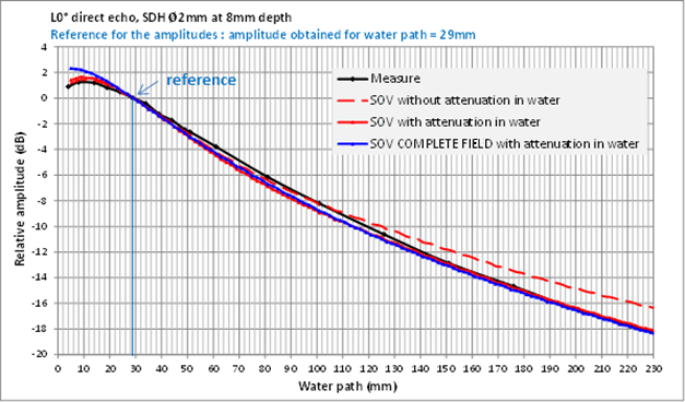
Figure 36 : Validation of the attenuation coefficient value in water by comparison with measured and with SOV and COMPLETE_SOV simulated amplitude/distance curves (with and without consideration of attenuation in water for SOV, with attenuation in water for COMPLETE_SOV). Ø2 mm SDH located at 8 mm depth in the stell calibration block, water path of 29 mm. Ø6.35 mm plane probe, 5 MHz.
reference for the amplitudes while MEaSURE/CIVA comparisons
The reference in amplitude for the experiment/CIVA comparisons is the amplitude af the L0° specular echo of the Ø2 mm SDH located at 8 mm depth inspected at a water path of 29 mm (Figure 35). As the with SOV and COMPLETE_SOV simulated amplitudes of this echo are similar (Figure 37), the same value in point has been used as reference for both models.
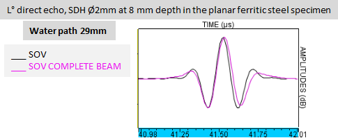
Figure 37 : Superimposition of with SOV and COMPLETE_SOV simulated A-scans of the reference SDH echo for the amplitudes (Ø2 mm located at 8 mm depth in a steel calibration block, water path 20 mm) showing that both models predict similar echoes. Comparables amplitudes. Ø6.35 mm plane probe, 5 MHz.
Beam of the 5 MHz probe in water
Figures 38 and 39 show the field emitted by the probe in water after a CIVA beam computation.
The maximal amplitude emitted by the probe on its axis is at a distance of 33.7 mm. The focal spot width at -3 dB is 1.9 mm at this distance (Figure 38).
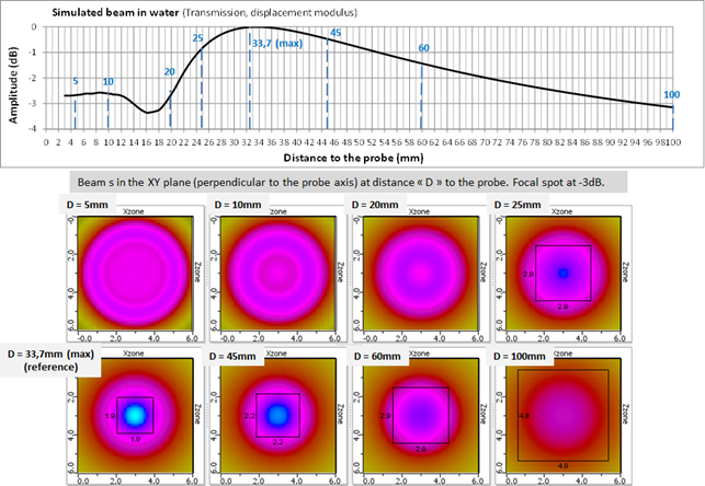
Figure 38 : Simulation with CIVA of the emitted field by the probe in water. On the top: field profile along the probe axis showing a maximum at 33.7 mm from the probe. On the bottom: field cartographies (6 mm x 6 mm) in planes perpendicular at its axis at different distances from the probe. Comparable amplitudes (ref = maximal field amplitude obtained at D = 33.7 mm). Ø6.35 mm plane probe, 5 MHz.
The Ø4 et 6 mm inclusions are also much greater than the focal spot (Figure 39). They are represented at the same scale of the cartography scale in order to show their dimensions relatively to the focal spot.
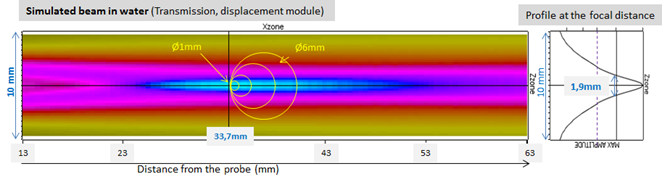
Figure 39 : CIVA simulation of the field emitted by the probe in water. Inclusions representation at the same scale of the cartography scale in order to show their dimensions relatively to the focal spot. Ø6.35 mm plane probe, 5 MHz.
results obtained for steel inclusions
In the table below are recalled CIVA restrictions for inclusions echoes with the 5 MHz probe. Those restrictions have been suppressed in the framework of this study in a development version in order to calculate the echoes of the 4 inclusions with the 3 SOV, COMPLETE_SOV and SPECULAR models. In the commercial version of CIVA, configurations corresponding to the “no” boxes in the Table 7 cannot be calculated due to these bridles.
|
5MHZ |
Ø 1mm |
Ø 2mm |
Ø 4mm |
Ø 6mm |
|
SOV |
yes |
no |
no |
no |
|
COMPLETE_SOV |
yes |
no |
no |
no |
|
SPECULAR |
no |
yes |
yes |
yes |
Table 7 : Available models in CIVA for inclusions echoes computations as a function of their diameter for the 5 MHz probe.
experimental results
The experimental amplitude/distance echodynamic curves obtained for the 4 inclusions are presented on the Figure 40. On the top, the amplitudes are relative to a reference echo amplitudes (SDH); on the bottom, the amplitudes are normalized. It can be noted that:
- the maximal amplitude of the echoes increases by 5 to 6 dB when the inclusion diameter is doubled. An increae of 2.5 dB is measured between the Ø4 et 6 mm inclusions.
- the « dmax » distance at which the echo amplitude is maximal has been recorded on the amplitude/distance curves. It depends quite not on the inclusion diameter: dmax varies from almost 32 mm to 34 mm (see following table).
- outside « dmax », the decreasing slope do not depend on the inclusion diameter.
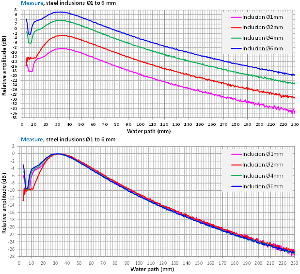
Figure 40 : Experimental results showing the amplitude/distance echodynamic curves with the steel inclusions diameters (1 to 6 mm). On the top: comparable amplitudes, reference: L0° echo of a Ø2 mm SDH at 8 mm depth, 29 mm water path. On the bottom: normalized amplitudes. Ø6.35 mm plane probe, 5 MHz.
The XY experimental curves obtained for the 4 inclusions at the experimental focal distances are presented on the Figure 4 (normalized amplitudes). The focal spot width do not depend on the inclusion diameter.
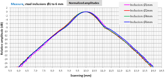
Figure 41 : Experimental results showing the evolution of the XY experimental cuts at the focal distance with the steel inclusions diameters (1 to 6 mm). Ø6.35 mm plane probe, 5 MHz.
The shape of the specular echoes of Ø1 to 6 mm inclusions located at the focal spot of 33.5 mm or in far fiels at 60 mm from the probe do not depend on the inclusions diameter (Figure 42). The echo arriving after the first contribution is even more far from the first echo than the inclusion diameter is great.
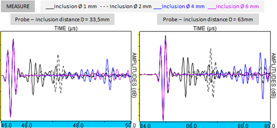
Figure 42 : Experimental results showing the XY experimental cuts evolution at the experimental focal disctance with the Ø1 mm to Ø6 mm isteel inclusions. Normalized amplitudes. Ø6.35 mm plane probe, 5 MHz.
MEaSURE/CIVA comparisons
-
Amplitude/distance curves
The comparisons of experimental and with SOV-COMPLETE, SOV and SPECULAR models simulated amplitude/distance curves are presented Figure 43 ( Ø1 mm and Ø2 mm inclusions) and Figure 44 (Ø4 mm and Ø6 mm inclusions).
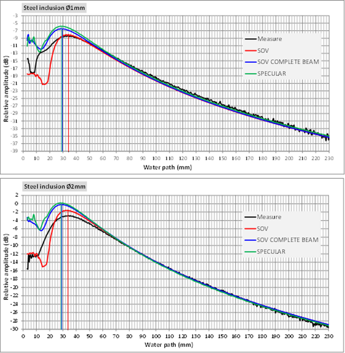
Figure 43 : Comparisons of experimental and with SOV, COMPLETE_SOV and SPECULAR models simulated amplitude/distance curves, Ø1 mm and Ø2 mm inclusions. The vertical lines corresponds to the maximal amplitude position emitted on the probe axis for each model. Reference for the amplitudes: L0° echo of a Ø2 mm SDH at 8 mm depth in a ferritic steel calibration block, 29 mm water path. In the commercial version of CIVA, the SOV and COMPLETE_SOV? models are allowed for the Ø1 mm inclusion and SPECULAR model is allowed for the Ø2 mm inclusion. Ø6.35 mm plane probe, 5 MHz.
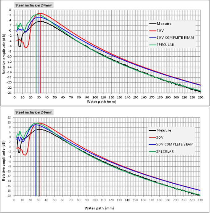
Figure 44 : Comparisons of experimental and with SOV, COMPLETE_SOV and SPECULAR models simulated amplitude/distance curves, Ø4 mm and Ø6 mm inclusions. The vertical lines corresponds to the maximal amplitude position emitted on the probe axis for each model. Reference for the amplitudes: L0° echo of a Ø2 mm SDH at 8 mm depth in a ferritic steel calibration block, 29 mm water path. In the commercial version of CIVA, only SPECULAR model is allowed for Ø4 mm and Ø6 mm inclusions. Capteur plan Ø6.35mm, 5MHz.
The dmax distance at which the amplitude/distance amplitude is maximal is indicated in the Table 8 for the measure and the 3 CIVA models.
|
Distance “D” of amp max (mm) |
Simulated beam |
Inclusion Ø1mm |
Inclusion Ø2mm |
Inclusion Ø4mm |
Inclusion Ø6mm |
|
|
33.5 |
|
|
|
|
|
Measure |
|
33.5 |
34 |
32.5 |
32 |
|
SOV |
|
34 |
33 |
32.5 |
31.5 |
|
COMPLETE_SOV_BEAM |
|
29 |
28.5 |
30.5 |
26.5 |
|
SPECULAR |
|
28.5 |
28 |
28 |
28 |
Table 8: Probe/inclusions distances (mm) corresponding at amplitude maximum emitted on the probe axis after the measure and the simulations with SOV, COMPLETE_SOV and SPECULAR models. The values written in bold correspond to the available cases in the commercial version of CIVA. Ø6.35 mm plane probe, 5 MHz.
Discrepancies between dmaxEXPERIMENTAL and dmaxCIVA are indicated in the Table 9.
|
Δdistance of amp max ΔDsim/exp (mm) |
Inclusion Ø1mm |
Inclusion Ø2mm |
Inclusion Ø4mm |
Inclusion Ø6mm |
|
SOV |
+0.5 |
-1 |
0 |
-0.5 |
|
COMPLETE_SOV_BEAM |
-4.5 |
-5.5 |
-2 |
-5.5 |
|
SPECULAR |
-5.5 |
-6 |
-4.5 |
-4 |
Table 9: Discrepancies between probe/inclusions distances (mm) corresponding to the measured and with SOV, COMPLETE_SOV and SPECULAR simulated amplitude maximum emitted on the probe axis. Differences (in mm) between the probe/inclusion distances corresponding to the experimental and simulated maximal amplitude emitted on the probe axis with SOV, COMPLETE_SOV and SPECULAR. The values written in bold correspond to the available cases in the commercial version of CIVA. Ø6.35 mm plane probe, 5 MHz.
- SOV Model : at small probe/inclusion distances, SOV predictions are not in agreement with the measure (particularly at distances smaller than dmax) and point out a SOV predictions instability.
The « dmax_SOV » distance is very close to dmax_experimental for all inclusions.
dmax_SOV depends on the inclusion diameter and varie by 31.5 to 34 mm (Table 8). Discrepancies between dmax_SOV and dmax_experimental are smaller than 1 mm (Table 9).
At great probe/inclusion distances, SOV model predictions are in agreement with the measure for the Ø1 mm and Ø2 mm inclusions. They are not in agreement for the Ø4 mm and Ø6 mm inclusions (overestimation reaching 2 dB for the Ø6 mm inclusion).
- COMPLETE_SOV model : small probe/inclusion distances, COMPLETE_SOV predictions are not in agreement with the measure: COMPLETE_SOV overestimates the amplitudes around dmax for all inclusions (from 2 to 3 dB).
The « dmax_COMPLETE_SOV » distance is far from dmax_experimental for all inclusions.
dmax_COMPLETE_SOV depends on the inclusion diameter and varies by 26.5 to 30.5 mm (Table 8). The differences between dmax_COMPLETE_SOV and dmax_experimental are important: COMPLETE_SOV overestimates dmax of 2 to 5.5mm (Table 9).
At great probe/inclusion distances, simulations are close to the one obtained with the SOV model at great distances. Consequently, they are far from the measure for the Ø4 mm and Ø6 mm inclusions (overestimation reaching 2 dB for the Ø6 mm inclusion).
- SPECULAR model : it gives results close to COMPLETE_SOV model results, exceept for the Ø4 mm and Ø6 mm inclusions amplitudes in far field which are well predicted by SPECULAR while COMPLETE_SOV overestimates them.
The « dmax_SPECULAR » distance is far from dmax_experimental for all inclusions.
dmax_SPECULAR does not depend on the inclusions diameter and is 28 mm (Table 8).
Discrepancies between dmax_ SPECULAR and dmax_experimental are important: SPECULAR overestimates dmax from 4 to 6 mm (Table 9).
Those measure/simulations comparisons point out:
- at small probe/inclusion distances, COMPLETE_SOV results are better than SOV results because COMPLETE_SOV eliminates some not valid approximations in the probe far field. However, as SOV results, they show important discrepancies with the measure. No error has been found and those observed discrepancies in far field have to be analyzed. It can be explained in part by the probe description and by the all models common hypothesis which considers that a probe surface vibration is « piston mode » like.
- The SPECULAR model prediction are good for the Ø4 mm and Ø6 mm inclusions echoes while both other models overestimate the amplitudes relatively to the measure. It is important to note that those SOV and COMPLETE_SOV bad predictions for the Ø4 mm and Ø6 mm inclusions echoes validates the restriction that allows only SPECULAR model for both inclusions.
- the bad predictions for dmax for COMPLETE_SOV and SPECULAR models (discrepancies reaching 6 mm).
An example of experimental and with SOV, COMPLETE_SOV and SPECULAR simulated A-scans of inclusions echoes are represented on the Figures 45 and 46 for different distances between probe and inclusion.
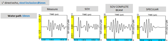
Figure 45 : Comparisons with experimental and with SOV, SCOMPLETE_SOV and SPECULAR simulated A-scans, Ø1 mm inclusion located at 10 mm from the probe on its axis. Ø6.35 mm plane probe, 5 MHz.
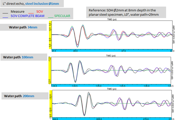
Figure 46 : Comparisons with experimental and with SOV, COMPLETE_SOV and SPECULAR simulated A-scans, Ø1 mm inclusion located at 34, 100 and 200 mm probe on its axis. Reference for the amplitudes: L0° echo of Ø2 mm inclusions located at 8 mm depth in a ferritic steel block, 29 mm water path. Ø6.35 mm plane probe, 5 MHz.
The specular echo is well predicted by the 3 models. The SOV and COMPLETE_SOV models also predict quite well the contribution coming after this echo when the probe/inclusion distance is great enough so that it is temporally separated from the specular echo. SPECULAR model does not simulate this contribution.
-
Cartographies in the XY plane at the focal distance
The « XY » experimental echodynamic curves extracted at the probe/inclusion distance of 34 mm (experimenal focal distance) are close to the one simulated with the 3 models almost 2 mm around their maximum (Figure 47). Beyond, the 3 models tends to under estimate the inclusions echoes amplitudes when they move away from the probe axis.
Warning : those curves are normalized in ampitude (max amplitude = 0 dB) in order to compare the focal widths.
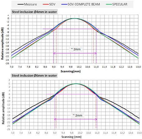
Figure 47 : Comparisons of measured and with SOV, COMPLETE_SOV and SPECULAR simulated XY curves, Ø4 mm and Ø6 mm inclusions. Normalized amplitudes. Ø6.35 mm planar probe, 5 MHz.
The focal spot width at -6 dB does almost not depend on the inclusion diameter, it is 2 mm according to the measure, value close to the one predicted by the 3 CIVA models.
Experimental and simulated (with SOV, COMPLETE_SOV and SPECULAR) A-scans of the 4 inclusions echoes are represented below. The inclusions are located at the experimental distance on the probe axis (A-scans at the left hand side of each figure) and at different increments (A-scans in the middle and at the right hand side).
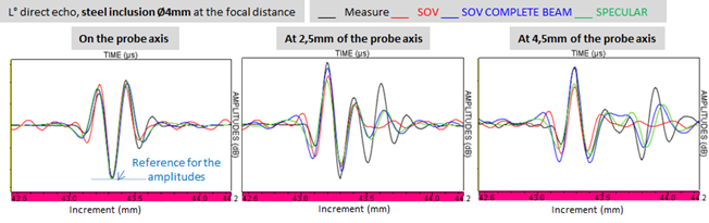
Figure 48 : Comparisons of measured and with SOV, SOV-COMPLET and SPECULAR simulated A-scans. Ø4 mm inclusion at the focal distance and at different increments. Normalized amplitudes when the inclusion is on the probe axis. Ø6.35 mm plane probe, 5 MHz.
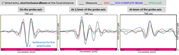
Figure 49 : Comparisons of measured and with SOV, COMPLETE_SOV and SPECULAR simulated A-scans. Ø6 mm inclusion at the focal distance and at different increments. Normalized amplitudes when the inclusion is on the probe axis. Ø6.35 mm plane probe, 5 MHz.
Those comparisons show that the 3 models predict similar echoes close to the measure exceept for the Ø6 mm inclusion and for the 6 mm shift (Figure 49, right hand side). COMPLETE_SOV and SPECULAR predictions are different from SOV predictions and are closer to the measure. This illustrates the contribution of the COMPLETE_SOV model relatively to SOV when the inclusion is shifted from the probe axis and that the «plane wave» approximation is not valid anymore.
Results obtained for the infinite plane
The comparisons of the experimental and with SPECULAR and KIRCHHOFF models simulated amplitude/distance curves (Figure 50) show a good agreement for the great water paths (> 70 mm). Both models overestimate the amplitudes by less than 2 dB. For smaller water paths, the overestimation does not exceed 3 dB.
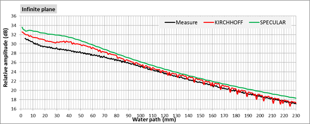
Figure 50 : Comparisons of the experimental and with SPECULAR and KIRCHHOFF models simulated amplitude/distance curves, infinite plane. Reference for the amplitudes: L0° echo of a Ø2 mm SDH at 8 mm depth in a ferritic steel calibration block, 29 mm water path. Ø6.35 mm plane probe, 5 MHz.
As the amplitudes, the measured and simulated (with SPECULAR and KIRCHHOFF) A-scans are slightly different at the small water paths but become very close at great water paths (Figure 51).
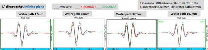
Figure 51 : Superimposition of measured and with SPECULAR and KIRCHHOFF simulated A-scans, infinite plane. Comparable amplitudes. Ø6.35 mm plane probe, 5 MHz.
Measured and simulated (with SPECULAR) A-scans have been represented on the Figure 52 in order to point out the good prediction of the phase evolution of the infinite plane echo when the probe/plane distance increases. It can also be seen on thoses figures that the A-scans predicted by the SPECULAR model have a lower frequency than the experimental A-scans.
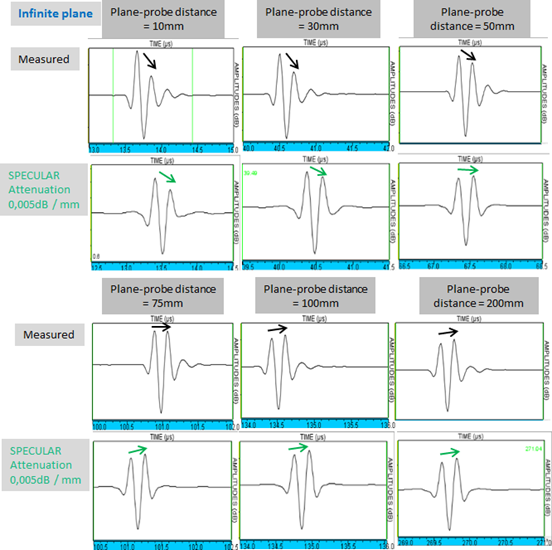
Figure 52 : Comparisons of the phase evolution of measured and with SPECULAR model simulated A-scans, infinite plane at different probe distances in water. Not comparable amplitudes. Ø6.35 mm plane probe, 5 MHz.
echoes spectrum of the inclusions and the infinite plane
Central frequency (fc) and bandwidth (BW) at -6 dB have been compared:
- measured and with SPECULAR and KIRCHHOFF spectra of the infinite plane placed at 33 mm (focal distance), 100 mm and 200 mm (far field) from the probe. Results are gathered in the Table 10.
- measured and with SOV, COMPLETE_SOV and SPECULAR Ø1 mm et Ø4 mm inclusions situated on the probe axis at 33.5 mm, 100 mm and 200 mm. The Ø1 mm inclusion results are reported in Table 11.
|
Infinite plane |
||||||
|
Distance probe/plane |
33mm |
100mm |
200mm |
|||
|
|
fc (MHz) |
BW (MHz) |
fc (MHz) |
BW (MHz) |
fc (MHz) |
BW (MHz) |
|
Measure |
4.7 |
3.3 |
5 |
3.5 |
4.9 |
3.3 |
|
SPECULAR |
4 |
3.1 |
4.3 |
3.2 |
4.3 |
3.2 |
|
KIRCHHOFF |
4.9 |
3.2 |
4.9 |
3.2 |
4.8 |
2.9 |
Table 10 : Comparisons of characteristics (fc and BW) from measured and with SOV, COMPLETE_SOV and SPECULAR simulated results of the spectrum of the infinite plane specular echoes in water at 33.5 mm, 100 mm and 200 mm from the probe. The values written in blod correspond to the non restricted cases in CIVA. Ø6.35 mm plane probe, 5 MHz.
|
Inclusion Ø4mm |
||||||
|
Distance probe/inclusion |
33mm |
100mm |
200mm |
|||
|
|
fc (MHz) |
BW (MHz) |
fc (MHz) |
BW (MHz) |
fc (MHz) |
BW (MHz) |
|
Measure |
4.5 |
2.8 |
5 |
3.25 |
4.9 |
3.2 |
|
SOV |
4.9 |
3.1 |
4.9 |
3.3 |
4.8 |
3.2 |
|
SOV-COMPLETE-BEAM |
4 |
2.7 |
4.8 |
3.2 |
4.7 |
3.2 |
|
SPECULAR |
3.9 |
2.8 |
4.4 |
3.2 |
4.3 |
3.1 |
Table 11: Comparisons of characteristics (fc and BW) from measured and with SOV, COMPLETE_SOV and SPECULAR simulated results of the spectrum of the Ø4 mm steel inclusion specular echoes in water at 33.5 mm, 100 mm and 200 mm from the probe. The values written in blod correspond to the non restricted cases in CIVA. Ø6.35 mm plane probe, 5 MHz.
Regarding the central frequency, those comparisons show that:
- For the infinite plane: an underestimation at the central frequency of the infinite plane echoes spectra with SPECULAR model, while KIRCHHOFF model correctly predicts those frequencies.
- For the inclusions:
- the central frequencies of SOV and COMPLETE_SOV models are the same at great distances. They generally are underestimated relatively to the experiment (max -0.5 MHz for the Ø1 mm non restricted inclusion in CIVA). On the other hand, at the focal distance 33 mm, COMPLETE_SOV predicts central frequencies lower than SOV (that can be seen on A-scans obtained with both models, figure 53) and that deviate from the measure.
- an underestimation of the central frequency of inclusions echoes spectra with SPECULAR model (as for the infinite plane)
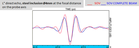
Figure 53 : Simulation results. Superimposition of with SOV and COMPLETE_SOV simulated A-scans with the Ø4 mm inclusion echo. Those comparisons show that SOV predicts an echo with greater frequency than COMPLETE_SOV at the probe focal distance. Comparable amplitudes. Ø6.35 mm plane probe, 5 MHz.
Regarding the bandwith:
- the echoes bandwith slightly varies around 3 MHz with the reflector and the distance from the probe is well predicted by all models.
EFFEcT of a poor variation in the central frequency
We evaluated the effect of a variation of 0.25MHz (5% of the center frequency “fc” equal to 5 MHz used in previous simulations) on the results of simulations.
To understand this effect on the echoes of the inclusions and the infinite plane, the good agreement experiment / simulation for the reference echo (SDHØ2mm at 8mm depth inspected with a water height of 19mm) for the 3 frequencies ( 4.75MHz, 5MHz and 5.25MHz) has been verified. Indeed, it is essential to allow the comparison measurement / simulation for other reflectors.
Figure 54 shows that the reference A-scan echoes simulated at three frequencies are in accordance with the measurement (Figure 54).
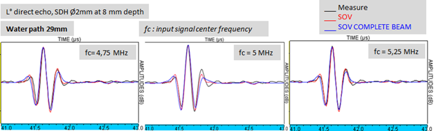
Figure 54 : Superposition of experimental and simulated A-scans with SOV and COMPLETE_SOV of the reference SDH echo. These comparisons show that simulated Ascans for central frequencies of 4.75, 5 and 5.25MHz are in good agreement with the experiment. Normalised amplitudes. Planar probe, Ø6.35mm, 5MHz.
The amplitude/distance curves simulated with SOV, COMPLETE_SOV and SPECULAR for the 3 frequencies have been plotted. Figure 55 shows the results for the Ø6mm inclusion. The reference for each curve amplitudes corresponds to the amplitude of the SDH echo at the same frequency.
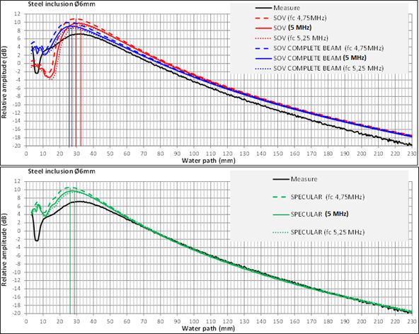
Figure 55 : Superposition of experimental and simulated (with SOV and COMPLETE_SOV (top) and SPECULAR (bottom) amplitude/distance curves for the Ø6mm inclusion. These comparisons show that the values and positions of the maximums of the amplitude/distance curves depend on the central frequency (4.75 MHz and 5.25 MHz). Planar probe, Ø6.35mm, 5MHz.
We noticed that the central frequency variation leads to a variation of the amplitudes of the inclusions around the maximal amplitude (2dB max.) and leads to a variation of the probe/inclusion distance ( around 2 mm) where is measured the maximal amplitude. These variations can be considered as simulation uncertainties linked to the uncertainty on the value of the central frequency of the entry signal.
Synthesys
For steel inclusions, at short distances probe / inclusion, all three models show results different from the experiments. Although COMPLETE_SOV makes fewer approximations than SOV in the near field, this is not enough to predict good amplitudes for inclusions located at small distances. Moreover discrepancies between measurement and COMPLETE_SOV for the maximum of the amplitude curves / distance position is very important. At large probe/inclusion distances,SOV and COMPLETE_SOV results are identical. They are consistent with the measurement for inclusions of 1 and 2 mm diameter but disagree for inclusions of Ø4m and Ø6mm which justifies the bridle currently present in CIVA (which allows for calculation of these inclusion echoes only the model SPECULAR). The center frequency spectrum of the inclusions echoes and of the infinite plane is generally underestimated by COMPLETE_SOV and SPECULAR models. The differences observed in this study are being analyzed.
Continue to Results with the 10 MHz focused probe
Back to Results with the 2.25 MHz probe
Back to Single element probe