
Inclusion in water – single element – Simulation settings
Summary
MODELS AND CIVA VERSIONS USED
STEEL SPHERICAL INCLUSIONS
The models that were used to calculate the steel spherical inclusion echoes located in water are:
- SOV (Separation Of Variables) with plane wave approximation for the incident field : it corresponds to the SOV model available in CIVA 2015a and previous versions
- SOV without plane wave approximation for the incident field. It is then called COMPLETE_SOV. The possibility to overcome the plane wave approximation is a new feature of CIVA 2016.
- SPECULAR
Given the assumptions and approximations related to each model, each one has its own domain of validity. The validity ranges depend on the ratio between the central frequency of the probe and the size of the spherical inclusion. The bridles are:
- for SOV and COMPLETE_SOV : bridle when k*radius>20 with k is the wave number. A warning is displayed and the simulation doesn’t run.
The test is performed with vL and/or vT according to the considered modes.
- for SPECULAR : warning when k*radius<20, but the calculation may be run.
The bridles interresting us are the ones listed below:
|
|
Ø 1mm |
Ø 2mm |
Ø 4mm |
Ø 6mm |
|
2.25MHZ |
|
|
|
|
|
SOV |
yes |
yes |
yes |
no |
|
COMPLETE_SOV |
yes |
yes |
yes |
no |
|
SPECULAR |
no |
no |
no |
yes |
|
5MHZ |
|
|
|
|
|
SOV |
yes |
no |
no |
no |
|
COMPLETE_SOV |
yes |
no |
no |
no |
|
SPECULAR |
no |
yes |
yes |
yes |
|
10MHZ |
|
|
|
|
|
SOV |
no |
no |
no |
no |
|
COMPLETE_SOV |
no |
no |
no |
no |
|
SPECULAR |
yes |
yes |
yes |
yes |
INFINITE PLAN
The model that has been used for the echoes calculation of the infinite plan is the SPECULAR model.
SIDE DRILLED HOLES AND FLAT BOTTOM HOLES
SDHs and FBHs were placed at different depths in calibation specimens.
In order to simulate SDHs echoes, SOV and COMPLETE_SOV models were used. There are no particular bridle with these reflectors and these models (SOV and COMPLETE_SOV) even if this model is known for not simulating accurately large SDHs.
KIRCHHOFF and COMPLETE_KIRCHHOFF models have been used to simulate FBHs echoes (COMPLETE means that there is no plane wave approximation for the incident beam on the defect, this a new feature of CIVA 2016). There are no particular bridle for the use of these models for FBHs.
NOTE: Some simulations were calculated with accuracy for beam and defect response equal to 10 in order to ensure the convergence of the results.
DETERMINATION OF SIGNAL PARAMETERS INPUT IN CIVA
In CIVA, the input parameters of a probe are the central frequency of signal, the bandwidth and the phase. For a given probe, these parameters are the same for all the calculation echoes model.
The central frequency of the entry signal is the nominal frequency of the probe with no modification following the adjustment below.
The adjustment of the central frequency is not performed because it may depend on the reference reflector used (SDH, FBH, surface echp,…) but also on the model chosen for the reference echo calculation (SOV, KIRCHHOFF, SPECULAR,…).This dependence is due to the fact that the echoes produced by different models for different reflectors are not completely “accurate” because of the assumptions and approximations associated with each model. In addition, inaccuracies “are found” in some way in the adjusted central frequency. Furthermore, the method also depends on the reliability of the reference echo acquisition.
If we take the example of the 5MHz immersion probe of Ø19mm diameter, the central frequency of the signal adjusted so L0° experimental and simulated echoes with COMPLETE_SOV model of the Ø2mm SDH loacted at 64mm depth and 50mm water path are in good agreement is 5.4 MHz (Figure 11) instead of 4.6 MHz with the SOV (Figure 10).
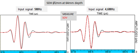
Figure 10 : Adjustment of the central frequency of the input signal so SOV simulated and experimental Ascans of a Ø2mm SDH located at 64mm depth in a steel block are in good agreement. Amplitudes normalisées. Flat immersion probe, Ø19mm, 5MHz, L0°, waterpath 50mm.
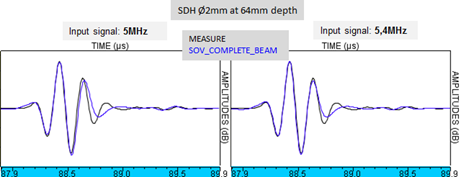
Figure 11 : Adjustment of the central frequency of the input signal so COMPLETE_SOV simulated and experimental Ascans of a Ø2mm SDH located at 64mm depth in a steel block are in good agreement. Amplitudes normalisées. Flat immersion probe, Ø19mm, 5MHz, L0°, waterpath 50mm.
Therefore, in order to avoid le dependance of the central frequency on the reflector’s nature and on the simulation model, the nominal frequency of the probe used in CIVA is not adjusted. The effect of a small variation of the central frequency on the simulation results is studied to evaluate the uncertianty associated with this parameter.
By contrast, the other two signal parameters (bandwidth and phase) are always determined by adjusting the temporal shapes of the measured and simulated echoes from a reference reflector which CIVA predictions has been validated.
DEterminING THE CURVATURE OF THE CRYSTAL OF THE FOCUSED PROBE WITH CIVA
The focused probe used for this study comprise a lens which curvature is unknow just like the wave celerity in the material. We modeled this probe by a focused shaped probe (without lens) which radius of curvature is determined so that the focal length in water provided by CIVA is equal to the one indicated by the manufacturer.
CIVA Configuration FOR THE simulation OF XZ OR YZ catographies
In CIVA, in order to simulate inclusions cartographies, a specimen which material is fluid (water) must be defined.
In addition, XZ cartographies are particular: CIVA allows to simulate them using a CAD of planar geometry (material is fluid), selecting the positioning according to the center of the probe’s crystal and the scanning as shown in Figure 12. Such cartography can not be simulated using a flat piece.
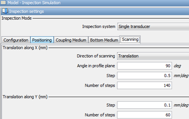
Figure 12 : Configuration of the scanning used for simulating XZ or YZ cartographies.
The amplitude /distance curves from the infinite plan are obtained by simulating the surface echo of a flat CAD specimen in the configuration described on Figure 12.
Note: in the case of the focused probe, the waterpath in CIVA corresponds to the height shown on Figure 13. It is measured from the center of the crystal.
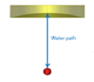
Figure 13 : Definition of the waterpath in CIVA for a focused probe without lens.
Continue to results obtained with the 2.25 MHz probe
Back to Experimental set-up
Back to Single element probe